Lecture 2: Data science pipeline Frame problems in the real world, we need to define and frame the problems first Collect data in the real world, you may need to collect data using
sensors, crowdsourcing, mobile apps. There are also other sources for getting public datasets, such as Hugging Face, Zenodo, Google Dataset Search, etc Preprocess Data Filtering →
can reduce a set of data based on specific criteria vb. left table can be reduced to the right table using a population threshold. df[df[“population”]>500000]. Aggregation → reduces a set
of data to a descriptive statistic. vb. left table is reduced to a single number by computing the mean value. df[“population”].mean(). Grouping → divides a table into groups by column
values, which can be chained with data aggregation to produce descriptive statistics for each group. vb. df.groupby(“province”).sum(). Sorting → rearranges data based on values in a
column, which can be useful for inspection. vb. right table is sorted by population. df.sort_values(by=[“population””]). Concatenation → combines multiple datasets that have the same
variables. vb. two left tables can be concatenated into the right table. pandas.concat([df_A, df_B]). Merging and joining → method to merge multiple data tables which have an
overlapping set of instances. vb. use “city” as the key to merge A and B. A.merge(B, how=”inner/left/right/outer”, on=”city”). Quantization → transforms a continuous set of values (e.g.
integers) into a discrete set (e.g. categories) . vb. age is quantized to age range. bin = [0,20,50,200]. L=[“1-20”, “21-50”, “51+”]. pandas.cut(D[“age”], bin, labels=L). Scaling → transforms
variables to have another distribution, which puts variables at the same scale and makes the data work better on many models. vb. Z-score scaling → represents how many standard
deviations from the mean. (df-df.mean()) / df.std(). vb. min-max scaling → making the value range between 0 and 1. (df-df.min()) / (df.max()-df.min()). Resample time series data to a
different frequency using different aggregation methods. vb. resample to hourly frequency using mean. df.resample(“60min”, label=”right”).mean(). Rolling → to transform time series
data using different aggregation methods. vb. df[“new_column”] = df[“column1”].rolling(window=3).sum(). Transformation → can be applied to rows or columns in a dataframe.
df[“wind_sine”] = np.sin(np.deg2rad(D[“wind_deg”])). Extract data → from text or match text patterns with regular expression → language to specify search patterns. vb. df[“year”] =
df[“venue”].str.extract(r’([0-9]{4})’). Drop → data we don’t need, such as duplicate data records or those that are irrelevant to our research question. pandas.drop(columns=[“year”]. can
drop rows or columns. Replace missing values → with a constant, mean, median or the most frequent value along the same column. constant imputation → -1. mean imputation. Model
missing values → where y is the variable/column that has the missing values, X means other variables, and F is a regression function. vb. y = F(X). different missing data may require
different data cleaning methods. MCAR → missing at completely random. missing data is completely random subset of the entire dataset. MAR → missing at random. missing data is
only related to variables other than the one having missing data. MNAR → Missing Not At Random. missing data is related to the variable that has the missing data. Explore data.
Information visualization is a good way for both experts and lay people to explore data and gain insights. python seaborn library to quickly plot and explore structure data. python plotly
library to build interactive visualizations. Voyant Tools to explore text data Model data. techniques for modeling structured, text, and image data through different modules image
classification. vb. optical character recognition → recognizing digits from hand-written images. vb. fine-grained categorization → categorizing the types of birds. text classification. vb.
sentiment analysis → identifying emotions from movie reviews. vb. categorizing the research aspect Deploy models can enable further quantitative or qualitative research with insights.
Data Science Fundamentals (Modeling). Classification. To classify spam messages we need examples → a dataset with observation (messages) and labels (spam or ham). We can
extract features (information) using human knowledge, which can help distinguish spam and ham messages. Using features x (which contains x1 and x2), we can represent each
message as one data point on a p-dimensional space (p=2 in this case). We can think of the model as a function f that can separate the observation into groups (labels y) according to
their features = {x1, x2}. f(x) > 0 → spam, f(x) < 0 → ham. To find a good function f, we start from f and train it until satisfied. We need something to tell us which direction and magnitude
to update. First, we need an error metric. vb. sum of distances between the misclassified points and line f. error = -y * f(x) for each misclassified point x={x1,x2}. We can use gradient
descent to minimize the error to train the model f iteratively. Depending on the needs, we can train different models (using different loss function) with various shapes and decision
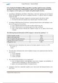
boundaries. To evaluate our classification model, we need to compute evaluation metrics to measure and quantify model performance. Accuracy = # of correctly classified points / # of all
points. Only works on a balanced dataset. Unbalanced dataset → accuracy for each class separately. If we care more about the positive class: precision = TP / (TP + FP) → how many
selected items are relevant. Recall = TP / (TP + FN) → how many relevant items are selected. F-Score = 2 * precision * recall / (precision + recall). To choose models, we need a test
set, which contains data that the models have not yet seen before during the training phase. To tune hyper-parameters or select features for a model, we use cross-validation to divide
the dataset into folds and use each fold for validation. Don’t use the test-set to tune hyper-parameters or select features, which will lead to information leakage. Training set → for training
models. Validation → for tuning hyper-parameters and/or selecting features. Way to select features → recursively eliminate the less important ones by using metrics like permutation
importance → permuting a feature several times and measuring the decrease in model performance. If two highly correlated features exist, the model can access the information from
the non-permuted feature. Thus, it may appear that both features are not important. A better way is to cluster the correlated features first. For time-series data, it is better to do the split
for cross-validation based on the order of time intervals, which means we only use data in the past to predict the future, but not the other way around. Regression. Fits a function that
maps features x to a continuous variable y. Linear regression → fits a linear function f that maps x1 (vb. the first feature vector of something) to y, which can best describe their linear
relationship. We can now create a feature matrix X that includes the intercept term 0, which gives us a compact form of equation. We can now generalize linear regression to have
multiple predictors and keep the compact mathematical representation. We use the vector and matrix forms to simplify equations. We can map vector and matrix forms to data directly.
We can look at the feature matrix X from two different directions: one represents the features → columns, one represents the data points → rows. Finally, we need an error metric
between the estimated response y and the true response y to know if the model fits the data well. Usually, we assume that the error e is IID (independent and identically distributed) and
follows a normal distribution with zero mean and some variance 2. To find the optimal coefficient, we need to minimize the error using gradient descent or taking the derivative of its matrix
form. We can model a non-linear relationship using a polynomial function with degree k. Using too complex/simple models can lead to overfitting/underfitting. The model fits the training
set well but generalizes poorly on the dataset. To evaluate regression models, one common metric is the coefficient of determination (R-squared). For simple/multiple linear regression,
R-squared equals the square of Pearson correlation coefficient r between the true y and the estimate y = f(X). R-squared increases as we add more predictors and thus is not a good
metric for model selection. The adjusted R-squared considers the number of samples (n) and predictors (p). A bad R-squared does not always mean no pattern in the data. A good
R-squared does not always mean that the function fits the data well. R-squared can be greatly affected by outliers. Lecture 3. Structured data generally means the type of data that has
standardized formats and well-defined structures. Mathematically speaking, we want to estimate a function f that can map feature X to label y such that prediction f(X) is close to y as
much as possible. Decision trees. Has a non-linear decision boundary that iteratively partitions the feature space. For simplicity, assume all features are binary. If we could only ask one
question, which question would we ask? We want to use the most useful feature that gives us the most information to help us guess. How can we quantify which features give the most
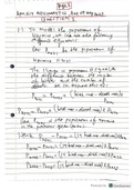
information? Misclassification error rates → 1 - #correct#voorbeeld / #fout#voorbeeld. Total error rate → nNo/nTotal * ENo + nYes/nTotal * EYes. vb: 80/100 * 10/80 + 0/20 * 20/100.
Entropy. Suppose we have a coin: one side has the label “stink,” and another side has the label “clean.” The entropy H intuitively means the averaged surprise when we flip this coin. H =
probability * Surprise. Surprise = log2(1/p). Entropy is zero when the coin always gives one side. Entropy reaches the maximum when the coin is fair, meaning both sides have equal
probability. When splitting the parent node, we can use the averaged entropy of the leaf node to measure and quantify the information that each feature gives. We can also use
information gain to measure the reduction in uncertainty after the split. Information Gain = Hparent - Hleaf. We can stop splitting when the information gain is too small for the best
feature, which means splitting the node does not give a reasonable reduction of error. Misclassification error is not the best method as the node-splitting strategy because it is not very
sensitive to changes in probabilities and can lead to zero information gain. Decision tree facts. Also works on continuous features but requires extra care. Can overfit easily. To combat →
we can stop splitting a node when it reaches the maximum tree depth or does not have a minimum sample size. Or → use the bagging technique → ensemble of multiple trees (Random
Forest model). Bagging technique for Random Forest model. Uses randomly selected features and bootstrapped samples (samples with replacement). The classifier that we trained is
one of all possible classifiers. We can sample many datasets D with pairs of features x and labels y. For all D, we can train a set of models. The generalization errors of a model can be
decomposed into bias, variance, and noise. Overfitting comes from training a very complex model that has a high variance. Both overfitting and underfitting mean that the model does not
generalize well on new data. In practice, we estimate the generalization error using a validation set. Overfitting usually happens when the model has a low training error but high
validation error. We can use the weak law of numbers to reduce the variance of a complex model. Bagging is one of the ensemble learning methods, where multiple weak classifiers are
combined into a strong classifier using various techniques. Not everything in the data is learnable → noise. PCA. Reducing the dimensions using PCA (Principal Components Analysis)
can be a good idea for reducing computational cost or visualizing data. Finds a new orthogonal coordinate system by rotating the axes to identify the directions that capture the largest
variation in the data. Minimizes the sum of squared perpendicular distances between the data points and the line, while linear regression minimizes the sum of squared vertical distances.
Form of unsupervised learning → no labeled data. Classification/regression is supervised learning → labeled data. Lecture 5. Deep learning is the idea of stacking different types of
layers to perform very complex tasks. Before the deep learning era, machine learning researchers needed to extract features from the data manually, but now we can delegate feature
engineering to the neural net. Instead of relying on manually crafted features, deep learning models can learn different representations from data automatically. Deep learning models
can extract features automatically and existed long ago but were not widespread due to the high demand for computational resources and power. For sequential data, we can use the
Recurrent Neural Network (RNN) architecture. For machine translation, the sequence-to-sequence model (which is an RNN) uses the encoder-decoder architecture. The encoder takes
the input in one language, and the decoder outputs the translation to another language. We can use Autoencoder (based on combining encoder-decoder architecture) to perform image
segmentation (using convolutional layers). A recent state-of-the-art is the Transformer architecture. We can also use deep learning to generate data, such as the Generative Adversarial
Network structure, which combines a generator (that converts noise to a fake sample) and a discriminator (that tries to identify if a sample is fake or real). Deep neural net. An artificial
neuron can convert feature x to prediction 𝑦 by using a weighted sum and an activation function. Then, we need to define a loss function based on the task type. We need to minimize the
error/cost to find the optimal parameter. We can represent the perceptron classifier using an artificial neuron. In this case, we use the identity function (as the activation) with the soft
perceptron loss. We have also learned linear regression, where we need to find a set of coefficients that can minimize the squared distances between all the predictions and ground
truths. We can also represent the linear regression model using an artificial neuron. In this case, we use the identity activation function with the squared error loss function. We can
replace the activation and loss functions with different ones to build another model. The example below uses hinge loss, which becomes Support Vector Machine. Support Vector
Machine (right figure) finds the maximum margin 𝛾 separating hyperplane h(x) for classification, while the perceptron classifier finds a separating hyperplane if it exists (e.g., blue or red
line on the left figure). Logistic Regression model. If we replace the activation function with sigmoid and use the logistic loss, the neuron becomes a Logistic Regression model. Fits a
logistic curve to the data to perform classification tasks. Training the deep neural network. We need to use optimization algorithms, such as gradient descent, to help us find a local
minimum (or global minimum for convex functions) on the cost function. We need to set a learning rate, which means the pace of moving forward for each update. Gradient is a
generalization of derivative. The intuition is that computing the derivative of 𝑓(𝑥) at point 𝑥^ means computing the slope of the tangent line to 𝑓(𝑥) at point 𝑥^. We need to adjust the
learning rate strategically. A large learning rate could lead to divergent behavior in the model. For example, the training loss could wiggle. How do we adjust the weight after computing
the loss for each iteration? To update the weights in previous layers, we need to use the backpropagation algorithm. Intuitively speaking, after comparing the prediction and the ground
truth, we want to increase the weight for the neuron we care about the most and decrease the others. We apply the same idea to iteratively update all the weights for all the neurons in
every previous layer, starting from the last layer, and backpropagate the errors back. In practice, we use mini-batches (instead of all data) when running gradient descent to increase the
speed (and save computer memory) when updating neuron weights. The backpropagation algorithm applies the chain rule in calculus to compute gradients. Overfitting deep neural
nets. We can combat overfitting by randomly dropping out neurons with a pre-defined probability (i.e., the dropout technique), which forces the model to avoid paying too much attention
to a particular set of features. We can also combat overfitting by using the regularization technique (also setting its strength factor 𝜆), which regulates model weights to ensure that they
sensors, crowdsourcing, mobile apps. There are also other sources for getting public datasets, such as Hugging Face, Zenodo, Google Dataset Search, etc Preprocess Data Filtering →
can reduce a set of data based on specific criteria vb. left table can be reduced to the right table using a population threshold. df[df[“population”]>500000]. Aggregation → reduces a set
of data to a descriptive statistic. vb. left table is reduced to a single number by computing the mean value. df[“population”].mean(). Grouping → divides a table into groups by column
values, which can be chained with data aggregation to produce descriptive statistics for each group. vb. df.groupby(“province”).sum(). Sorting → rearranges data based on values in a
column, which can be useful for inspection. vb. right table is sorted by population. df.sort_values(by=[“population””]). Concatenation → combines multiple datasets that have the same
variables. vb. two left tables can be concatenated into the right table. pandas.concat([df_A, df_B]). Merging and joining → method to merge multiple data tables which have an
overlapping set of instances. vb. use “city” as the key to merge A and B. A.merge(B, how=”inner/left/right/outer”, on=”city”). Quantization → transforms a continuous set of values (e.g.
integers) into a discrete set (e.g. categories) . vb. age is quantized to age range. bin = [0,20,50,200]. L=[“1-20”, “21-50”, “51+”]. pandas.cut(D[“age”], bin, labels=L). Scaling → transforms
variables to have another distribution, which puts variables at the same scale and makes the data work better on many models. vb. Z-score scaling → represents how many standard
deviations from the mean. (df-df.mean()) / df.std(). vb. min-max scaling → making the value range between 0 and 1. (df-df.min()) / (df.max()-df.min()). Resample time series data to a
different frequency using different aggregation methods. vb. resample to hourly frequency using mean. df.resample(“60min”, label=”right”).mean(). Rolling → to transform time series
data using different aggregation methods. vb. df[“new_column”] = df[“column1”].rolling(window=3).sum(). Transformation → can be applied to rows or columns in a dataframe.
df[“wind_sine”] = np.sin(np.deg2rad(D[“wind_deg”])). Extract data → from text or match text patterns with regular expression → language to specify search patterns. vb. df[“year”] =
df[“venue”].str.extract(r’([0-9]{4})’). Drop → data we don’t need, such as duplicate data records or those that are irrelevant to our research question. pandas.drop(columns=[“year”]. can
drop rows or columns. Replace missing values → with a constant, mean, median or the most frequent value along the same column. constant imputation → -1. mean imputation. Model
missing values → where y is the variable/column that has the missing values, X means other variables, and F is a regression function. vb. y = F(X). different missing data may require
different data cleaning methods. MCAR → missing at completely random. missing data is completely random subset of the entire dataset. MAR → missing at random. missing data is
only related to variables other than the one having missing data. MNAR → Missing Not At Random. missing data is related to the variable that has the missing data. Explore data.
Information visualization is a good way for both experts and lay people to explore data and gain insights. python seaborn library to quickly plot and explore structure data. python plotly
library to build interactive visualizations. Voyant Tools to explore text data Model data. techniques for modeling structured, text, and image data through different modules image
classification. vb. optical character recognition → recognizing digits from hand-written images. vb. fine-grained categorization → categorizing the types of birds. text classification. vb.
sentiment analysis → identifying emotions from movie reviews. vb. categorizing the research aspect Deploy models can enable further quantitative or qualitative research with insights.
Data Science Fundamentals (Modeling). Classification. To classify spam messages we need examples → a dataset with observation (messages) and labels (spam or ham). We can
extract features (information) using human knowledge, which can help distinguish spam and ham messages. Using features x (which contains x1 and x2), we can represent each
message as one data point on a p-dimensional space (p=2 in this case). We can think of the model as a function f that can separate the observation into groups (labels y) according to
their features = {x1, x2}. f(x) > 0 → spam, f(x) < 0 → ham. To find a good function f, we start from f and train it until satisfied. We need something to tell us which direction and magnitude
to update. First, we need an error metric. vb. sum of distances between the misclassified points and line f. error = -y * f(x) for each misclassified point x={x1,x2}. We can use gradient
descent to minimize the error to train the model f iteratively. Depending on the needs, we can train different models (using different loss function) with various shapes and decision
boundaries. To evaluate our classification model, we need to compute evaluation metrics to measure and quantify model performance. Accuracy = # of correctly classified points / # of all
points. Only works on a balanced dataset. Unbalanced dataset → accuracy for each class separately. If we care more about the positive class: precision = TP / (TP + FP) → how many
selected items are relevant. Recall = TP / (TP + FN) → how many relevant items are selected. F-Score = 2 * precision * recall / (precision + recall). To choose models, we need a test
set, which contains data that the models have not yet seen before during the training phase. To tune hyper-parameters or select features for a model, we use cross-validation to divide
the dataset into folds and use each fold for validation. Don’t use the test-set to tune hyper-parameters or select features, which will lead to information leakage. Training set → for training
models. Validation → for tuning hyper-parameters and/or selecting features. Way to select features → recursively eliminate the less important ones by using metrics like permutation
importance → permuting a feature several times and measuring the decrease in model performance. If two highly correlated features exist, the model can access the information from
the non-permuted feature. Thus, it may appear that both features are not important. A better way is to cluster the correlated features first. For time-series data, it is better to do the split
for cross-validation based on the order of time intervals, which means we only use data in the past to predict the future, but not the other way around. Regression. Fits a function that
maps features x to a continuous variable y. Linear regression → fits a linear function f that maps x1 (vb. the first feature vector of something) to y, which can best describe their linear
relationship. We can now create a feature matrix X that includes the intercept term 0, which gives us a compact form of equation. We can now generalize linear regression to have
multiple predictors and keep the compact mathematical representation. We use the vector and matrix forms to simplify equations. We can map vector and matrix forms to data directly.
We can look at the feature matrix X from two different directions: one represents the features → columns, one represents the data points → rows. Finally, we need an error metric
between the estimated response y and the true response y to know if the model fits the data well. Usually, we assume that the error e is IID (independent and identically distributed) and
follows a normal distribution with zero mean and some variance 2. To find the optimal coefficient, we need to minimize the error using gradient descent or taking the derivative of its matrix
form. We can model a non-linear relationship using a polynomial function with degree k. Using too complex/simple models can lead to overfitting/underfitting. The model fits the training
set well but generalizes poorly on the dataset. To evaluate regression models, one common metric is the coefficient of determination (R-squared). For simple/multiple linear regression,
R-squared equals the square of Pearson correlation coefficient r between the true y and the estimate y = f(X). R-squared increases as we add more predictors and thus is not a good
metric for model selection. The adjusted R-squared considers the number of samples (n) and predictors (p). A bad R-squared does not always mean no pattern in the data. A good
R-squared does not always mean that the function fits the data well. R-squared can be greatly affected by outliers. Lecture 3. Structured data generally means the type of data that has
standardized formats and well-defined structures. Mathematically speaking, we want to estimate a function f that can map feature X to label y such that prediction f(X) is close to y as
much as possible. Decision trees. Has a non-linear decision boundary that iteratively partitions the feature space. For simplicity, assume all features are binary. If we could only ask one
question, which question would we ask? We want to use the most useful feature that gives us the most information to help us guess. How can we quantify which features give the most
information? Misclassification error rates → 1 - #correct#voorbeeld / #fout#voorbeeld. Total error rate → nNo/nTotal * ENo + nYes/nTotal * EYes. vb: 80/100 * 10/80 + 0/20 * 20/100.
Entropy. Suppose we have a coin: one side has the label “stink,” and another side has the label “clean.” The entropy H intuitively means the averaged surprise when we flip this coin. H =
probability * Surprise. Surprise = log2(1/p). Entropy is zero when the coin always gives one side. Entropy reaches the maximum when the coin is fair, meaning both sides have equal
probability. When splitting the parent node, we can use the averaged entropy of the leaf node to measure and quantify the information that each feature gives. We can also use
information gain to measure the reduction in uncertainty after the split. Information Gain = Hparent - Hleaf. We can stop splitting when the information gain is too small for the best
feature, which means splitting the node does not give a reasonable reduction of error. Misclassification error is not the best method as the node-splitting strategy because it is not very
sensitive to changes in probabilities and can lead to zero information gain. Decision tree facts. Also works on continuous features but requires extra care. Can overfit easily. To combat →
we can stop splitting a node when it reaches the maximum tree depth or does not have a minimum sample size. Or → use the bagging technique → ensemble of multiple trees (Random
Forest model). Bagging technique for Random Forest model. Uses randomly selected features and bootstrapped samples (samples with replacement). The classifier that we trained is
one of all possible classifiers. We can sample many datasets D with pairs of features x and labels y. For all D, we can train a set of models. The generalization errors of a model can be
decomposed into bias, variance, and noise. Overfitting comes from training a very complex model that has a high variance. Both overfitting and underfitting mean that the model does not
generalize well on new data. In practice, we estimate the generalization error using a validation set. Overfitting usually happens when the model has a low training error but high
validation error. We can use the weak law of numbers to reduce the variance of a complex model. Bagging is one of the ensemble learning methods, where multiple weak classifiers are
combined into a strong classifier using various techniques. Not everything in the data is learnable → noise. PCA. Reducing the dimensions using PCA (Principal Components Analysis)
can be a good idea for reducing computational cost or visualizing data. Finds a new orthogonal coordinate system by rotating the axes to identify the directions that capture the largest
variation in the data. Minimizes the sum of squared perpendicular distances between the data points and the line, while linear regression minimizes the sum of squared vertical distances.
Form of unsupervised learning → no labeled data. Classification/regression is supervised learning → labeled data. Lecture 5. Deep learning is the idea of stacking different types of
layers to perform very complex tasks. Before the deep learning era, machine learning researchers needed to extract features from the data manually, but now we can delegate feature
engineering to the neural net. Instead of relying on manually crafted features, deep learning models can learn different representations from data automatically. Deep learning models
can extract features automatically and existed long ago but were not widespread due to the high demand for computational resources and power. For sequential data, we can use the
Recurrent Neural Network (RNN) architecture. For machine translation, the sequence-to-sequence model (which is an RNN) uses the encoder-decoder architecture. The encoder takes
the input in one language, and the decoder outputs the translation to another language. We can use Autoencoder (based on combining encoder-decoder architecture) to perform image
segmentation (using convolutional layers). A recent state-of-the-art is the Transformer architecture. We can also use deep learning to generate data, such as the Generative Adversarial
Network structure, which combines a generator (that converts noise to a fake sample) and a discriminator (that tries to identify if a sample is fake or real). Deep neural net. An artificial
neuron can convert feature x to prediction 𝑦 by using a weighted sum and an activation function. Then, we need to define a loss function based on the task type. We need to minimize the
error/cost to find the optimal parameter. We can represent the perceptron classifier using an artificial neuron. In this case, we use the identity function (as the activation) with the soft
perceptron loss. We have also learned linear regression, where we need to find a set of coefficients that can minimize the squared distances between all the predictions and ground
truths. We can also represent the linear regression model using an artificial neuron. In this case, we use the identity activation function with the squared error loss function. We can
replace the activation and loss functions with different ones to build another model. The example below uses hinge loss, which becomes Support Vector Machine. Support Vector
Machine (right figure) finds the maximum margin 𝛾 separating hyperplane h(x) for classification, while the perceptron classifier finds a separating hyperplane if it exists (e.g., blue or red
line on the left figure). Logistic Regression model. If we replace the activation function with sigmoid and use the logistic loss, the neuron becomes a Logistic Regression model. Fits a
logistic curve to the data to perform classification tasks. Training the deep neural network. We need to use optimization algorithms, such as gradient descent, to help us find a local
minimum (or global minimum for convex functions) on the cost function. We need to set a learning rate, which means the pace of moving forward for each update. Gradient is a
generalization of derivative. The intuition is that computing the derivative of 𝑓(𝑥) at point 𝑥^ means computing the slope of the tangent line to 𝑓(𝑥) at point 𝑥^. We need to adjust the
learning rate strategically. A large learning rate could lead to divergent behavior in the model. For example, the training loss could wiggle. How do we adjust the weight after computing
the loss for each iteration? To update the weights in previous layers, we need to use the backpropagation algorithm. Intuitively speaking, after comparing the prediction and the ground
truth, we want to increase the weight for the neuron we care about the most and decrease the others. We apply the same idea to iteratively update all the weights for all the neurons in
every previous layer, starting from the last layer, and backpropagate the errors back. In practice, we use mini-batches (instead of all data) when running gradient descent to increase the
speed (and save computer memory) when updating neuron weights. The backpropagation algorithm applies the chain rule in calculus to compute gradients. Overfitting deep neural
nets. We can combat overfitting by randomly dropping out neurons with a pre-defined probability (i.e., the dropout technique), which forces the model to avoid paying too much attention
to a particular set of features. We can also combat overfitting by using the regularization technique (also setting its strength factor 𝜆), which regulates model weights to ensure that they