Overzicht begrippen week 1-3
Lecture 2
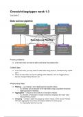
Data science pipeline
Frame problems
● in the real world, we need to define and frame the problems first
Collect data
● in the real world, you may need to collect data using sensors, crowdsourcing, mobile
apps
● There are also other sources for getting public datasets, such as Hugging Face,
Zenodo, Google Dataset Search, etc
Preprocess Data
● Filtering → can reduce a set of data based on specific criteria
○ vb. left table can be reduced to the right table using a population threshold
○ df[df[“population”]>500000]
● Aggregation → reduces a set of data to a descriptive statistic
○ vb. left table is reduced to a single number by computing the mean value
○ df[“population”].mean()
● Grouping → divides a table into groups by column values, which can be chained
with data aggregation to produce descriptive statistics for each group
○ vb. df.groupby(“province”).sum()
, ● Sorting → rearranges data based on values in a column, which can be useful for
inspection
○ vb. right table is sorted by population
○ df.sort_values(by=[“population””])
● Concatenation → combines multiple datasets that have the same variables
○ vb. two left tables can be concatenated into the right table
○ pandas.concat([df_A, df_B])
● Merging and joining → method to merge multiple data tables which have an
overlapping set of instances
○ vb. use “city” as the key to merge A and B
○ A.merge(B, how=”inner/left/right/outer”, on=”city”)
● Quantization → transforms a continuous set of values (e.g. integers) into a discrete
set (e.g. categories)
○ vb. age is quantized to age range
○ bin = [0,20,50,200]
○ L=[“1-20”, “21-50”, “51+”]
○ pandas.cut(D[“age”], bin, labels=L)
● Scaling → transforms variables to have another distribution, which puts variables at
the same scale and makes the data work better on many models
○ vb. Z-score scaling → represents how many standard deviations from the
mean
○ (df-df.mean()) / df.std()
○ vb. min-max scaling → making the value range between 0 and 1
○ (df-df.min()) / (df.max()-df.min())
● Resample time series data to a different frequency using different aggregation
methods
○ vb. resample to hourly frequency using mean
○ df.resample(“60min”, label=”right”).mean()
● Rolling → to transform time series data using different aggregation methods
○ vb. df[“new_column”] = df[“column1”].rolling(window=3).sum()
● Transformation → can be applied to rows or columns in a dataframe
○ df[“wind_sine”] = np.sin(np.deg2rad(D[“wind_deg”]))
● Extract data → from text or match text patterns with regular expression → language
to specify search patterns


