Week 1 Lecture: Multiple Linear Regression
Part 1: frequentist vs bayesian statistics.
There are 2 possible statistical frameworks for data analysis:
The frequentist framework focuses on assessing how well the observed data fit the
null hypothesis (H⁰) (NHST= Null hypothesis significance testing). Key tools include p-values
(the probability of obtaining the observed data, or more extreme results, assuming H⁰ is
true), confidence intervals (ranges likely to contain the true parameter value under repeated
sampling), effect sizes (the magnitude of an observed effect), and power analysis (the
probability of detecting a true effect given the study design). Frequentist methods rely solely
on the observed data and do not incorporate prior information.
In contrast, the Bayesian framework calculates the probability of a hypothesis given
the data, explicitly incorporating prior beliefs. It updates these prior beliefs with the observed
data to produce a posterior distribution. Tools like Bayes factors (BFs) quantify the evidence
for one hypothesis over another, while credible intervals provide a range where a parameter
likely falls, based on the posterior. Bayesian methods allow for integrating prior knowledge
and provide a direct probabilistic interpretation of results.
In the frequentist framework you can make a frequentist estimation.
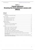
Empirical research uses collected data to learn from. Information from this
data is captured in a likelihood function. It indicates how likely different
parameter values (e.g., population mean: μ) explain the observed data. The
red dots are the data and in the middle they are more close to each other so
there will be the high of the function. The probability of the likelihood in the
extremes is low. The likelihood function says ‘the probability of the data given
μ’. In the frequentist estimation all relevant information for inference is
contained in the likelihood function.
In the Bayesian approach when we make a likelihood function we may also have
prior information about μ. The central idea/mechanism of Bayesian is: ‘prior knowledge is
updated with information in the data and together provides the posterior distribution from μ.
- The advantage is: accumulating knowledge (‘today’s posterior is tomorrow’s prior).
- The disadvantage is that the results depend on prior
choices.
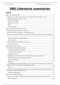
The prior influences the posterior, when we have no idea how the
function is and we get the data then the line will almost be the
same as the data but when we have an idea and we gain new
data then the line will change more confidently in the direction of
the data. For example we first thought the blue line, then the
brown data came and now we have more confidence so the
posterior line is black. The posterior distribution (line) of the
parameters of interest provides all desired estimates:
- Posterior mean or mode: the mean or mode of the posterior distribution
- Posterior SD: SD (standard deviation) of posterior distribution (comparable to
frequentist standard error)
- Posterior 95% credible interval: providing the bounds of the part of the posterior
with 95% of the posterior mass
This makes Bayesian estimates.
,When testing hypotheses with a frequentist framework you have an H⁰ and if the p-value is
below 0.05 you reject H⁰ and take H¹. With bayesian testing you take previous attempts into
account and the results depend on things not observed on the sampling plan, which means
the same data can give different results. This is because frequentist frameworks
and bayesian frameworks have different definitions of probability:
- Frequentist: testing conditions on H⁰ with a p-value; probability of
observing same or more extreme data given that the null is true (data|H⁰).
This is really low if you look at all the dead people and how many are
dead because of a shark.
- Bayesian: Bayes conditions on observed data, probability that
hypothesis is supported by the data (H|data). This is really high, if
someone has gotten their head bit off the probability of them being dead
is really high.
When testing hypotheses, bayesians can calculate the probability of the
hypothesis given the data. This is called PMP (posterior model probability); the bayesian
probability of the hypothesis after observing the data.
The bayesian probability of a hypothesis being true depends on 2 criteria:
1. How sensible it is, based on prior knowledge (the prior)
2. How well it fits the new evidence (the data).
Bayesian hypothesis testing is comparative: hypotheses are tested against each other, not
in isolation. This means hypothesis 1 or 0 is as many times stronger/weaker than the other
one. You can see it in the bayes factor formula. A BF¹⁰=10 means that
hypothesis 1 is 10 times stronger than hypothesis 0. A BF¹⁰ =1 means that
hypothesis 1 is equal as strong as hypothesis 0. A BF⁰¹=10 means that
hypothesis 0 is 10 times stronger than hypothesis 1. The first number after BF is
what is stronger/weaker. PMP’s (posterior probabilities of hypotheses are also
called relative probabilities. PMP are updates of prior probabilities (for hypotheses) with
the BF.
Both frameworks use probability theory:
- Frequentist: probability is the relative frequency of events (more formal?)
- Bayesian: probability is the degree of belief (more intuitive?)
This leads to debate (same word for different things) and to differences in the correct
interpretation of statistical results (for example p-value vs PMP). The main difference is:
- Frequentist 95% confidence interval (CI): if we were to repeat this experiment
many times and calculate a confidence interval each time, 95% of the intervals will
include the true parameter value (and 5% won’t). It’s about the long-term frequency
of the interval, not the probability of the true value being within a single interval.
- Bayesian 95% credible interval: There is 95% probability that the true value is in
the credible interval. The credible interval is a direct statement about the uncertainty
of the parameter value.
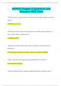
A linear regression is when 2 variables are against each other, one (y) dependent
and one (x) independent variable. The goal is to find a linear relationship between
the variables that can be represented by a straight line. You can make a scatterplot
for the scores on the variables x and y and the linear positive association between
,them. You use the formula for the blue line and the black formula for each point. In that
formula you see in red ‘ei’ which is the difference between the blue line and the black dots
and stands for error. The other name is residual and each black point has its own residual
and is the distance to the regression line. To fix it we look at the sum of all the squared
residuals and we want that number to be minimal. The regression line needs to be
minimizing the number of the squared residuals.
A multiple linear regression is a model with 1 dependent
variable and 2 or more independent variables. In multiple
regression there are a few assumptions. All results are only
reliable if assumptions made by the model and approach
roughly hold, in this case its: MLR assumes interval/ratio
variables (outcome and predictors).
Watch out:
- Serious violations lead to incorrect results
- Sometimes there are easy solutions (e.g. deleting a severe outlier; or adding a
quadratic term)
- Per model, know what assumptions are and always check them carefully
When you want to test a dichotomous/nominal variable (not interval/ratio) you can use
dummy variables as predictors. A dummy variable is a numerical representation of a
categorical variable that has two or more categories. For dichotomous variables (e.g.,
"Yes/No" or "Male/Female"), the variable is coded as 0 or 1.
When we put it in this formula we can treat it as a normal
categorical variable. The interpretation of B² is the difference
in mean grade between males and females with the same
age.
Evaluating the models:
Frequentist approaches do estimate the parameters of the model. They test with
NHST if parameters are significantly not zero. We can be interested in one side of the
hypothesis (whether H⁰ is true or false, it does not mean if H⁰ is false that H¹ is true). It simply
suggests there is evidence inconsistent with H⁰, but it does not quantify how much more
likely H¹ is compared to H⁰(this is a strength of Bayesian methods).
Bayesian statistical approaches estimate the parameters of the model. They
compare support in data for different models/hypotheses using Bayes factors. It provides a
direct measure of how much more likely one hypothesis is compared to another, based on
the observed data.
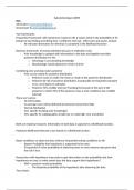
Output of the models:
The output of the frequentist analysis has 3 tables. First, we look at R², which is called the
coefficient of determination and is a measure of how well the model explains the variability of
the dependent variable (variance). The number is between 0 and 1. We also look at R which
is the multiple correlation coefficient, a measure of the strength and direction of the linear
relationship between two variables. We can also look at the adjusted R² and that is a
modified version of R² that adjusts for the number of predictors in a regression model. It
, accounts for the fact that adding more predictors to a model will always increase R²,
regardless of whether those predictors are truly
meaningful.
Table 1 →
In the second table we look at whether the amount
of explained variance is statistically significant.
Firstly, you look at the F-value which
compares the ratio of variance
explained by the model (due to
predictors) to the variance
unexplained (residual error). We also
look at the p-value, which in most
cases needs to be below an alpha 0.05 for it to be significant.
In the third and last table we see
the individual predictors of the
dependent variable. We look at
the p-values of the variables to
see if they are even significant.
Then you look at the
unstandardized coefficients
that are the raw coefficients (β)
that represent the relationship
between each predictor variable
and the dependent variable, measured in their original units. The unstandardized coefficient
indicates how much the dependent variable (Y) changes, on average, for a one-unit
increase in the predictor variable (X), while keeping other predictors constant.
We also look at the standardized coefficients which have been scaled so that they are
unitless. They represent the relative strength and direction of the relationship between each
predictor and the dependent variable in a regression model. Standardizing makes the
coefficients comparable across predictors.
The output in bayesian statistics is
different, we get 2 tables. The first is called
model comparison. The null model is a
model with B^age=0 and B^education=0.
Model 1 is where the predictors age and
education are included. Then you look at
BF¹⁰ and it gives you the Bayes factors.
The BF¹⁰=28.181 implies that the data are 28x more likely under model 1 than under the null
model.
The second table is called the posterior summary table. We see the effects of the individual
predictors. Bayesian estimates are
summary of posterior distribution
of parameters. Differences with
frequentist results can be explained
Part 1: frequentist vs bayesian statistics.
There are 2 possible statistical frameworks for data analysis:
The frequentist framework focuses on assessing how well the observed data fit the
null hypothesis (H⁰) (NHST= Null hypothesis significance testing). Key tools include p-values
(the probability of obtaining the observed data, or more extreme results, assuming H⁰ is
true), confidence intervals (ranges likely to contain the true parameter value under repeated
sampling), effect sizes (the magnitude of an observed effect), and power analysis (the
probability of detecting a true effect given the study design). Frequentist methods rely solely
on the observed data and do not incorporate prior information.
In contrast, the Bayesian framework calculates the probability of a hypothesis given
the data, explicitly incorporating prior beliefs. It updates these prior beliefs with the observed
data to produce a posterior distribution. Tools like Bayes factors (BFs) quantify the evidence
for one hypothesis over another, while credible intervals provide a range where a parameter
likely falls, based on the posterior. Bayesian methods allow for integrating prior knowledge
and provide a direct probabilistic interpretation of results.
In the frequentist framework you can make a frequentist estimation.
Empirical research uses collected data to learn from. Information from this
data is captured in a likelihood function. It indicates how likely different
parameter values (e.g., population mean: μ) explain the observed data. The
red dots are the data and in the middle they are more close to each other so
there will be the high of the function. The probability of the likelihood in the
extremes is low. The likelihood function says ‘the probability of the data given
μ’. In the frequentist estimation all relevant information for inference is
contained in the likelihood function.
In the Bayesian approach when we make a likelihood function we may also have
prior information about μ. The central idea/mechanism of Bayesian is: ‘prior knowledge is
updated with information in the data and together provides the posterior distribution from μ.
- The advantage is: accumulating knowledge (‘today’s posterior is tomorrow’s prior).
- The disadvantage is that the results depend on prior
choices.
The prior influences the posterior, when we have no idea how the
function is and we get the data then the line will almost be the
same as the data but when we have an idea and we gain new
data then the line will change more confidently in the direction of
the data. For example we first thought the blue line, then the
brown data came and now we have more confidence so the
posterior line is black. The posterior distribution (line) of the
parameters of interest provides all desired estimates:
- Posterior mean or mode: the mean or mode of the posterior distribution
- Posterior SD: SD (standard deviation) of posterior distribution (comparable to
frequentist standard error)
- Posterior 95% credible interval: providing the bounds of the part of the posterior
with 95% of the posterior mass
This makes Bayesian estimates.
,When testing hypotheses with a frequentist framework you have an H⁰ and if the p-value is
below 0.05 you reject H⁰ and take H¹. With bayesian testing you take previous attempts into
account and the results depend on things not observed on the sampling plan, which means
the same data can give different results. This is because frequentist frameworks
and bayesian frameworks have different definitions of probability:
- Frequentist: testing conditions on H⁰ with a p-value; probability of
observing same or more extreme data given that the null is true (data|H⁰).
This is really low if you look at all the dead people and how many are
dead because of a shark.
- Bayesian: Bayes conditions on observed data, probability that
hypothesis is supported by the data (H|data). This is really high, if
someone has gotten their head bit off the probability of them being dead
is really high.
When testing hypotheses, bayesians can calculate the probability of the
hypothesis given the data. This is called PMP (posterior model probability); the bayesian
probability of the hypothesis after observing the data.
The bayesian probability of a hypothesis being true depends on 2 criteria:
1. How sensible it is, based on prior knowledge (the prior)
2. How well it fits the new evidence (the data).
Bayesian hypothesis testing is comparative: hypotheses are tested against each other, not
in isolation. This means hypothesis 1 or 0 is as many times stronger/weaker than the other
one. You can see it in the bayes factor formula. A BF¹⁰=10 means that
hypothesis 1 is 10 times stronger than hypothesis 0. A BF¹⁰ =1 means that
hypothesis 1 is equal as strong as hypothesis 0. A BF⁰¹=10 means that
hypothesis 0 is 10 times stronger than hypothesis 1. The first number after BF is
what is stronger/weaker. PMP’s (posterior probabilities of hypotheses are also
called relative probabilities. PMP are updates of prior probabilities (for hypotheses) with
the BF.
Both frameworks use probability theory:
- Frequentist: probability is the relative frequency of events (more formal?)
- Bayesian: probability is the degree of belief (more intuitive?)
This leads to debate (same word for different things) and to differences in the correct
interpretation of statistical results (for example p-value vs PMP). The main difference is:
- Frequentist 95% confidence interval (CI): if we were to repeat this experiment
many times and calculate a confidence interval each time, 95% of the intervals will
include the true parameter value (and 5% won’t). It’s about the long-term frequency
of the interval, not the probability of the true value being within a single interval.
- Bayesian 95% credible interval: There is 95% probability that the true value is in
the credible interval. The credible interval is a direct statement about the uncertainty
of the parameter value.
A linear regression is when 2 variables are against each other, one (y) dependent
and one (x) independent variable. The goal is to find a linear relationship between
the variables that can be represented by a straight line. You can make a scatterplot
for the scores on the variables x and y and the linear positive association between
,them. You use the formula for the blue line and the black formula for each point. In that
formula you see in red ‘ei’ which is the difference between the blue line and the black dots
and stands for error. The other name is residual and each black point has its own residual
and is the distance to the regression line. To fix it we look at the sum of all the squared
residuals and we want that number to be minimal. The regression line needs to be
minimizing the number of the squared residuals.
A multiple linear regression is a model with 1 dependent
variable and 2 or more independent variables. In multiple
regression there are a few assumptions. All results are only
reliable if assumptions made by the model and approach
roughly hold, in this case its: MLR assumes interval/ratio
variables (outcome and predictors).
Watch out:
- Serious violations lead to incorrect results
- Sometimes there are easy solutions (e.g. deleting a severe outlier; or adding a
quadratic term)
- Per model, know what assumptions are and always check them carefully
When you want to test a dichotomous/nominal variable (not interval/ratio) you can use
dummy variables as predictors. A dummy variable is a numerical representation of a
categorical variable that has two or more categories. For dichotomous variables (e.g.,
"Yes/No" or "Male/Female"), the variable is coded as 0 or 1.
When we put it in this formula we can treat it as a normal
categorical variable. The interpretation of B² is the difference
in mean grade between males and females with the same
age.
Evaluating the models:
Frequentist approaches do estimate the parameters of the model. They test with
NHST if parameters are significantly not zero. We can be interested in one side of the
hypothesis (whether H⁰ is true or false, it does not mean if H⁰ is false that H¹ is true). It simply
suggests there is evidence inconsistent with H⁰, but it does not quantify how much more
likely H¹ is compared to H⁰(this is a strength of Bayesian methods).
Bayesian statistical approaches estimate the parameters of the model. They
compare support in data for different models/hypotheses using Bayes factors. It provides a
direct measure of how much more likely one hypothesis is compared to another, based on
the observed data.
Output of the models:
The output of the frequentist analysis has 3 tables. First, we look at R², which is called the
coefficient of determination and is a measure of how well the model explains the variability of
the dependent variable (variance). The number is between 0 and 1. We also look at R which
is the multiple correlation coefficient, a measure of the strength and direction of the linear
relationship between two variables. We can also look at the adjusted R² and that is a
modified version of R² that adjusts for the number of predictors in a regression model. It
, accounts for the fact that adding more predictors to a model will always increase R²,
regardless of whether those predictors are truly
meaningful.
Table 1 →
In the second table we look at whether the amount
of explained variance is statistically significant.
Firstly, you look at the F-value which
compares the ratio of variance
explained by the model (due to
predictors) to the variance
unexplained (residual error). We also
look at the p-value, which in most
cases needs to be below an alpha 0.05 for it to be significant.
In the third and last table we see
the individual predictors of the
dependent variable. We look at
the p-values of the variables to
see if they are even significant.
Then you look at the
unstandardized coefficients
that are the raw coefficients (β)
that represent the relationship
between each predictor variable
and the dependent variable, measured in their original units. The unstandardized coefficient
indicates how much the dependent variable (Y) changes, on average, for a one-unit
increase in the predictor variable (X), while keeping other predictors constant.
We also look at the standardized coefficients which have been scaled so that they are
unitless. They represent the relative strength and direction of the relationship between each
predictor and the dependent variable in a regression model. Standardizing makes the
coefficients comparable across predictors.
The output in bayesian statistics is
different, we get 2 tables. The first is called
model comparison. The null model is a
model with B^age=0 and B^education=0.
Model 1 is where the predictors age and
education are included. Then you look at
BF¹⁰ and it gives you the Bayes factors.
The BF¹⁰=28.181 implies that the data are 28x more likely under model 1 than under the null
model.
The second table is called the posterior summary table. We see the effects of the individual
predictors. Bayesian estimates are
summary of posterior distribution
of parameters. Differences with
frequentist results can be explained