Stanford CS229: Machine Learning
Amrit Kandasamy
November 2024
1 Linear Regression and Gradient Descent
Lecture Note Slides
1.1 Notation and Definitions
Pn
Linear Regression Hypothesis: hθ (x) = i=0 θi xi , where x0 = 1.
θ0
..
θ= .
θn
is called the parameters of the learning algorithm. The algorithm’s job is to
choose θ.
x0
..
x= .
xn
is an input vector (often the inputs are called features).
We let m be the number of training examples (elements in the training set).
y is the output, sometimes called the target variable.
(x, y) is one training example. We will use the notation
(x(i) , y (i) )
to denote the ith training example.
As used in the vectors and summation n is the number of features.
:= denotes assignment (usually of some variable or function). For example,
a := a + 1 increments a by 1.
We write hθ (x) as h(x) for convenience.
1
, Figure 1: Visual of Gradient Descent with Two Parameters
1.2 How to Choose Parameters θ
Choose θ such that h(x) ≈ y for the training examples. Generally, we want to
minimize
m
1X
J(θ) = (hθ (x(i) ) − y)2
2 i=1
In order to minimize J(θ), we will employ Batch Gradient Descent.
Let’s look an example with 2 parameters. Start with some point (θ0 , θ1 , J(θ)),
determined either randomly or by some condition. We look around all around
and think,
”What direction should we take a tiny step in to go downward as fast as possible?”.
If a different starting point was used, the resulting optimum minima would have
been changed (see the two paths above).
Now let’s formalize the gradient descent algorithm(s).
1.2.1 Batch Gradient Descent
Let α be the learning rate. Then the algorithm can be written as
∂
θj := θj − α J(θ)
∂θj
Let’s derive the partial derivative part. Assume there’s only 1 training example
for now. Substituting our definition of J, we have
n
!
∂ ∂ 1 2 ∂ X
α J(θ) = (hθ (x) − y) = (hθ (x) − y) · ( θ i xi ) − y
∂θj ∂θj 2 ∂θj i=0
2
Amrit Kandasamy
November 2024
1 Linear Regression and Gradient Descent
Lecture Note Slides
1.1 Notation and Definitions
Pn
Linear Regression Hypothesis: hθ (x) = i=0 θi xi , where x0 = 1.
θ0
..
θ= .
θn
is called the parameters of the learning algorithm. The algorithm’s job is to
choose θ.
x0
..
x= .
xn
is an input vector (often the inputs are called features).
We let m be the number of training examples (elements in the training set).
y is the output, sometimes called the target variable.
(x, y) is one training example. We will use the notation
(x(i) , y (i) )
to denote the ith training example.
As used in the vectors and summation n is the number of features.
:= denotes assignment (usually of some variable or function). For example,
a := a + 1 increments a by 1.
We write hθ (x) as h(x) for convenience.
1
, Figure 1: Visual of Gradient Descent with Two Parameters
1.2 How to Choose Parameters θ
Choose θ such that h(x) ≈ y for the training examples. Generally, we want to
minimize
m
1X
J(θ) = (hθ (x(i) ) − y)2
2 i=1
In order to minimize J(θ), we will employ Batch Gradient Descent.
Let’s look an example with 2 parameters. Start with some point (θ0 , θ1 , J(θ)),
determined either randomly or by some condition. We look around all around
and think,
”What direction should we take a tiny step in to go downward as fast as possible?”.
If a different starting point was used, the resulting optimum minima would have
been changed (see the two paths above).
Now let’s formalize the gradient descent algorithm(s).
1.2.1 Batch Gradient Descent
Let α be the learning rate. Then the algorithm can be written as
∂
θj := θj − α J(θ)
∂θj
Let’s derive the partial derivative part. Assume there’s only 1 training example
for now. Substituting our definition of J, we have
n
!
∂ ∂ 1 2 ∂ X
α J(θ) = (hθ (x) − y) = (hθ (x) − y) · ( θ i xi ) − y
∂θj ∂θj 2 ∂θj i=0
2