Gauss Curvature and the Gauss-Bonnet Theorem
⃗ : 𝐷 → ℝ3 , be a smooth parametrized surface 𝑆 (𝛷
Let 𝛷 ⃗ (𝐷) = 𝑆, 𝑇
⃗𝑢 × 𝑇
⃗ 𝑣 ≠ 0).
We want to develop a definition of the Gauss Curvature of a surface at a point
𝑝 ∈ 𝑆.
Let’s start with 2 curves in the 𝑥, 𝑦 plane: 𝑦 = 𝑥 2 and 𝑦 = 4𝑥 2 .
𝑦 = 4𝑥 2
𝑦 = 𝑥2
Our intuition tells us that the curvature of 𝑦 = 4𝑥 2 at the point (0,0) is larger
than the curvature of 𝑦 = 𝑥 2 at (0,0). We can also intuitively conclude that the
notion of curvature should be related to the second derivative of the function at
that point. Not surprisingly, 𝑦’’ = 8 for the curve 𝑦 = 4𝑥 2 𝑎𝑡 (0,0), and 𝑦’’ = 2
for the curve 𝑦 = 𝑥 2 at (0,0). (In this particular example, the curvature of the 2
curves actually does equal 8 and 2, however, in general, the calculation of
curvature is a more complicated than just calculating the 2nd derivative.)
, 2
Now let’s parametrize both curves:
𝑐1 (𝑡 ) =< 𝑡, 𝑡 2 >
⃗⃗⃗ 𝑐2 (𝑡 ) =< 𝑡, 4𝑡 2 >
⃗⃗⃗
𝑐1 ′(𝑡 ) =< 1,2𝑡 > 𝑐2 ′(𝑡) =< 1, 8𝑡 >
𝑐1 ′′(𝑡 ) =< 0,2 > 𝑐2 ′′(𝑡) =< 0,8 >
Notice the upward pointing unit normal vector at the point (0,0) to both curves is
𝑛⃗ =< 0,1 >.
Finally, notice that the “curvatures” we calculated above can be gotten by:
𝑐1 ′′(𝑡) ∙ 𝑛⃗ =< 0,2 >∙< 0,1 > = 2
𝑐2 ′′(𝑡) ∙ 𝑛⃗ =< 0,8 >∙< 0,1 > = 8.
Thus it should not surprise us to see 2nd derivatives dotted with a unit normal
vector in a formula for curvature of a surface.
To define curvature for a surface we start by defining:
⃗⃗⃗ 2
𝜕𝛷 ⃗⃗⃗
𝜕𝛷 ⃗⃗⃗
𝜕𝛷 ⃗⃗⃗ 2
𝜕𝛷
𝐸=| | , 𝐹= ∙ , 𝐺=| |
𝜕𝑢 𝜕𝑢 𝜕𝑣 𝜕𝑣
It can be shown through a messy calculation that:
2
⃗𝑢 × 𝑇
|𝑇 ⃗ 𝑣 | = 𝐸𝐺 − 𝐹 2 .
Let 𝑊= 𝐸𝐺 − 𝐹 2 .
⃗⃗⃗ on the surface 𝑆 is given by:
We know that a unit normal vector, 𝑛,
⃗𝑢 × 𝑇
𝑇 ⃗𝑣 ⃗𝑢 × 𝑇
𝑇 ⃗𝑣
𝑛⃗ = = .
⃗ ⃗
|𝑇𝑢 × 𝑇𝑣 | √𝑊
⃗ : 𝐷 → ℝ3 , be a smooth parametrized surface 𝑆 (𝛷
Let 𝛷 ⃗ (𝐷) = 𝑆, 𝑇
⃗𝑢 × 𝑇
⃗ 𝑣 ≠ 0).
We want to develop a definition of the Gauss Curvature of a surface at a point
𝑝 ∈ 𝑆.
Let’s start with 2 curves in the 𝑥, 𝑦 plane: 𝑦 = 𝑥 2 and 𝑦 = 4𝑥 2 .
𝑦 = 4𝑥 2
𝑦 = 𝑥2
Our intuition tells us that the curvature of 𝑦 = 4𝑥 2 at the point (0,0) is larger
than the curvature of 𝑦 = 𝑥 2 at (0,0). We can also intuitively conclude that the
notion of curvature should be related to the second derivative of the function at
that point. Not surprisingly, 𝑦’’ = 8 for the curve 𝑦 = 4𝑥 2 𝑎𝑡 (0,0), and 𝑦’’ = 2
for the curve 𝑦 = 𝑥 2 at (0,0). (In this particular example, the curvature of the 2
curves actually does equal 8 and 2, however, in general, the calculation of
curvature is a more complicated than just calculating the 2nd derivative.)
, 2
Now let’s parametrize both curves:
𝑐1 (𝑡 ) =< 𝑡, 𝑡 2 >
⃗⃗⃗ 𝑐2 (𝑡 ) =< 𝑡, 4𝑡 2 >
⃗⃗⃗
𝑐1 ′(𝑡 ) =< 1,2𝑡 > 𝑐2 ′(𝑡) =< 1, 8𝑡 >
𝑐1 ′′(𝑡 ) =< 0,2 > 𝑐2 ′′(𝑡) =< 0,8 >
Notice the upward pointing unit normal vector at the point (0,0) to both curves is
𝑛⃗ =< 0,1 >.
Finally, notice that the “curvatures” we calculated above can be gotten by:
𝑐1 ′′(𝑡) ∙ 𝑛⃗ =< 0,2 >∙< 0,1 > = 2
𝑐2 ′′(𝑡) ∙ 𝑛⃗ =< 0,8 >∙< 0,1 > = 8.
Thus it should not surprise us to see 2nd derivatives dotted with a unit normal
vector in a formula for curvature of a surface.
To define curvature for a surface we start by defining:
⃗⃗⃗ 2
𝜕𝛷 ⃗⃗⃗
𝜕𝛷 ⃗⃗⃗
𝜕𝛷 ⃗⃗⃗ 2
𝜕𝛷
𝐸=| | , 𝐹= ∙ , 𝐺=| |
𝜕𝑢 𝜕𝑢 𝜕𝑣 𝜕𝑣
It can be shown through a messy calculation that:
2
⃗𝑢 × 𝑇
|𝑇 ⃗ 𝑣 | = 𝐸𝐺 − 𝐹 2 .
Let 𝑊= 𝐸𝐺 − 𝐹 2 .
⃗⃗⃗ on the surface 𝑆 is given by:
We know that a unit normal vector, 𝑛,
⃗𝑢 × 𝑇
𝑇 ⃗𝑣 ⃗𝑢 × 𝑇
𝑇 ⃗𝑣
𝑛⃗ = = .
⃗ ⃗
|𝑇𝑢 × 𝑇𝑣 | √𝑊