Lecture 1 oklog123
↑
prerequisites test Remindo
log (ab) log logb
=
a +
expla+ b) =
expa
.
expb exp(a b) .
=
expab
Regression recap: hypothesis = true function
Supervised learning where each datapoint is of the form x, t (t ∈ R) and we look for a hypothesis s.t. t ≈ f(x)
T
Linear regression: we look for a hypothesis s.t. t ≈ x * w
X matrix allows us to fit polynomials of degree up to K —> For N datapoints we have N rows, each column is a feature
Learned from bias-variance analysis/VC-dimension: smaller hypothesis class may mean better generalisation
performance
Overfitting: algorithm is allowed to pick too complex hypotheses (fits random noise too well at expense of fitting true
function underlying the data) continuous spectrum
of hypotheses
Another way to avoid too complex hypotheses: Regularisation (soft constraint) from simple to complex -
Instead of finding the weight vector w that minimises squared error: Loss function 2 ((Xw -t)T(Xw t) = -
We’ll find the one minimising the Penalised loss 2 2 + XwTw penalty =
—> If fitting the data requires large weights, algorithm can pick them, as long as the increase in penalty is offset by
enough reduction in loss (lambda λ is used to control trade-off between penalty and loss)
K-fold cross validation to find a good trade-off
We want to validate each value of λ on each of the K folds, and average those K results for each λ
Finding the optimal regularised w: Take partial derivative with respect to w of the penalised loss formula, set
expression to zero and solve for w —> w (X X NXI)" XTt = regularised least squares solution
=
+
+
X = [] Ex =
= 1
,
x =
polynomial degrees (feature 1)
Xi = X ....... X first column ;
only is
2 / ((Xw t)T(Xw t)
=
-
- + xwiw
2 : X Xw-
*
YNWX - + *
XWiw
+
wr + w =
2 = 2X Xw -
YwX
+
t + 2xw
*
set to zero+X Xw- Y X +
+ + 2xw = 0
w(2/NXTX 2x1) 2X t
+
-
=
*
w (2 X + X- 2x1)" Ex E
=
:
(X +X NXl)" X t
+
? w = - .
(XTX NX1) X t
+
+ =
w = (XTX + NX1) "XTt
, Lecture 2 07 109123
A different way to look at linear regression:
1) zoom in on how the data might be generated; looking at the probability distribution the data may be drawn from
Reason backward (generated data) to the true function we want to figure out
We determine the distribution, and if our model is close enough to reality, it may be useful (do realise that noise plays a
role in prediction)
Goal: learn how to predict a good t, when given x —> Focus on conditional distribution p(t1,…,tN | X) for N points
throw
Probability distributions: 5X
/(0-5)
:
P = probability, p = density & P(Y = y)
event : random variable
Property of a PDF is that it’s continuous
value
X
neads
= 2 means ; 2/5 throws landed heads
density >
-
probability
Mean: true function’s value for t at x ( P(T = 10.25 | X = 1980) = 0 )
Variance: usually unknown, oh
p (t Ez en) p(z) p(tz) p(tn) P(En) =
= ·
....
,,
Probabilistic independence:
...
,
Dependent random variables; x, y depend on each other (knowing value of x gives info on y)
Independent random variables; we look at PDF of x and y separately -> p(x , y) = p(x)p(y)
Dependent variables are necessary for us to be able to learn anything from training data points about new data
Independent noise: the noise terms ε: tn f(Xn) + En where f is the true function (randomly sample x, compute t, add noise)
=
Information in tn that’s relevant for predicting other t’s should be captured in f
The info in εn should be irrelevant for predicting other t’s —> noise terms are independent
! Conditional independence (x conditionally independent of y, given z: p(x, y | z) = p(x|z)p(y|z)
Conditional independence between the t’s, given f, σ2, and X allows us to write
-> and we decided that the distribution should be Gaussian with mean f(xn) and variance σ2
or Xn)
Ctrly , ,
During regression we have data (x & t) but don’t know f or σ2 —> we look for the f for which our data would have been
most likely
We look at a likelihood function L as a function of f and σ2 while we hold data fixed
Note: in linear regression we’re not looking for an arbitrary function f, but one that can be described by
a weigtht vector w s.t. f(x) = xT * w
Expression likelihood for single data point: L exp)-1/202 (tn -x w(2)
+
To express the likelihood we use a formula, which we can simplify by taking the logarithm (big product->big sum)
*log is monotonically increasing, so paramaters w and σ2 that maximise L will also maximise log L
! To maximize likelihood we take the derivative of log L, set it to 0 and get: = (XiX) "XIE ,which is the same w that
minimized squared loss
We can also find the max likelihood of σ2 by setting the log formula to zero with respect to o
! Solution: 2 = /Netn-Mw)2
which measures avg squared deviation of tn from its mean (analogous to def of variance)
The larger the difference between predictions and data, the larger σ2 gets
To know for sure that the calculated ‘derivative set to zero’ is a maximum we can check that the 2nd derivative is
negative (check slide)
For functions of vectors, we need the Hessian (matrix of second partial derivatives) to be negative definite (slide 21!!)
This means all eigenvalues need to be negative
Hessian of the likelihood w/ respect to w is 20 XX
*
ziX Xz0
-
-
We need to check that for all z = 0
2X'X20
-
So each square is > 0, so the sum is also > 0 and only 0 if all squares are 0
1
(Xz)"
N
X2 > 0
So, only in rare cases, our w is indeed the weight vector that maximizes likelihood
(x2)n0
likelihood
Maximizing minimizing regularized least
squares solution
find parameter values that observed data most probable find
make
parameter values that minize [cerrors' between predicted/observed
values constant to avoid
overfitting
+
reg .
↑
prerequisites test Remindo
log (ab) log logb
=
a +
expla+ b) =
expa
.
expb exp(a b) .
=
expab
Regression recap: hypothesis = true function
Supervised learning where each datapoint is of the form x, t (t ∈ R) and we look for a hypothesis s.t. t ≈ f(x)
T
Linear regression: we look for a hypothesis s.t. t ≈ x * w
X matrix allows us to fit polynomials of degree up to K —> For N datapoints we have N rows, each column is a feature
Learned from bias-variance analysis/VC-dimension: smaller hypothesis class may mean better generalisation
performance
Overfitting: algorithm is allowed to pick too complex hypotheses (fits random noise too well at expense of fitting true
function underlying the data) continuous spectrum
of hypotheses
Another way to avoid too complex hypotheses: Regularisation (soft constraint) from simple to complex -
Instead of finding the weight vector w that minimises squared error: Loss function 2 ((Xw -t)T(Xw t) = -
We’ll find the one minimising the Penalised loss 2 2 + XwTw penalty =
—> If fitting the data requires large weights, algorithm can pick them, as long as the increase in penalty is offset by
enough reduction in loss (lambda λ is used to control trade-off between penalty and loss)
K-fold cross validation to find a good trade-off
We want to validate each value of λ on each of the K folds, and average those K results for each λ
Finding the optimal regularised w: Take partial derivative with respect to w of the penalised loss formula, set
expression to zero and solve for w —> w (X X NXI)" XTt = regularised least squares solution
=
+
+
X = [] Ex =
= 1
,
x =
polynomial degrees (feature 1)
Xi = X ....... X first column ;
only is
2 / ((Xw t)T(Xw t)
=
-
- + xwiw
2 : X Xw-
*
YNWX - + *
XWiw
+
wr + w =
2 = 2X Xw -
YwX
+
t + 2xw
*
set to zero+X Xw- Y X +
+ + 2xw = 0
w(2/NXTX 2x1) 2X t
+
-
=
*
w (2 X + X- 2x1)" Ex E
=
:
(X +X NXl)" X t
+
? w = - .
(XTX NX1) X t
+
+ =
w = (XTX + NX1) "XTt
, Lecture 2 07 109123
A different way to look at linear regression:
1) zoom in on how the data might be generated; looking at the probability distribution the data may be drawn from
Reason backward (generated data) to the true function we want to figure out
We determine the distribution, and if our model is close enough to reality, it may be useful (do realise that noise plays a
role in prediction)
Goal: learn how to predict a good t, when given x —> Focus on conditional distribution p(t1,…,tN | X) for N points
throw
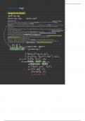
Probability distributions: 5X
/(0-5)
:
P = probability, p = density & P(Y = y)
event : random variable
Property of a PDF is that it’s continuous
value
X
neads
= 2 means ; 2/5 throws landed heads
density >
-
probability
Mean: true function’s value for t at x ( P(T = 10.25 | X = 1980) = 0 )
Variance: usually unknown, oh
p (t Ez en) p(z) p(tz) p(tn) P(En) =
= ·
....
,,
Probabilistic independence:
...
,
Dependent random variables; x, y depend on each other (knowing value of x gives info on y)
Independent random variables; we look at PDF of x and y separately -> p(x , y) = p(x)p(y)
Dependent variables are necessary for us to be able to learn anything from training data points about new data
Independent noise: the noise terms ε: tn f(Xn) + En where f is the true function (randomly sample x, compute t, add noise)
=
Information in tn that’s relevant for predicting other t’s should be captured in f
The info in εn should be irrelevant for predicting other t’s —> noise terms are independent
! Conditional independence (x conditionally independent of y, given z: p(x, y | z) = p(x|z)p(y|z)
Conditional independence between the t’s, given f, σ2, and X allows us to write
-> and we decided that the distribution should be Gaussian with mean f(xn) and variance σ2
or Xn)
Ctrly , ,
During regression we have data (x & t) but don’t know f or σ2 —> we look for the f for which our data would have been
most likely
We look at a likelihood function L as a function of f and σ2 while we hold data fixed
Note: in linear regression we’re not looking for an arbitrary function f, but one that can be described by
a weigtht vector w s.t. f(x) = xT * w
Expression likelihood for single data point: L exp)-1/202 (tn -x w(2)
+
To express the likelihood we use a formula, which we can simplify by taking the logarithm (big product->big sum)
*log is monotonically increasing, so paramaters w and σ2 that maximise L will also maximise log L
! To maximize likelihood we take the derivative of log L, set it to 0 and get: = (XiX) "XIE ,which is the same w that
minimized squared loss
We can also find the max likelihood of σ2 by setting the log formula to zero with respect to o
! Solution: 2 = /Netn-Mw)2
which measures avg squared deviation of tn from its mean (analogous to def of variance)
The larger the difference between predictions and data, the larger σ2 gets
To know for sure that the calculated ‘derivative set to zero’ is a maximum we can check that the 2nd derivative is
negative (check slide)
For functions of vectors, we need the Hessian (matrix of second partial derivatives) to be negative definite (slide 21!!)
This means all eigenvalues need to be negative
Hessian of the likelihood w/ respect to w is 20 XX
*
ziX Xz0
-
-
We need to check that for all z = 0
2X'X20
-
So each square is > 0, so the sum is also > 0 and only 0 if all squares are 0
1
(Xz)"
N
X2 > 0
So, only in rare cases, our w is indeed the weight vector that maximizes likelihood
(x2)n0
likelihood
Maximizing minimizing regularized least
squares solution
find parameter values that observed data most probable find
make
parameter values that minize [cerrors' between predicted/observed
values constant to avoid
overfitting
+
reg .