Unit 3: Scarcity, Wellbeing and Working Hours
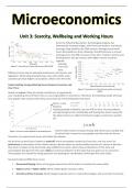
Since the Industrial Revolution, technological progress has
dramatically increased wages, with American workers' real hourly
earnings rising sixfold in the 20th century. Average annual work
hours decreased by a third, allowing a fourfold increase in annual
earnings and a one-fifth increase in free time. Trends in income and
working hours vary by country, with higher-income countries
typically
enjoying
Figure 3.1: Annual hours of work and income (1870–2018). more free
time.
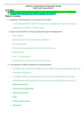
Differences arise due to individual preferences, job choices, and
legislation. While living standards have risen since 1870, some
countries prioritize higher consumption, others more free time.
Understanding Varying Working Hours Between Countries and
Over Time: Figure 3.2: Annual hours of free time per worker and income
(2020).
Goods are scarce if they are valued, and there is an opportunity
cost of acquiring more of them; this is a recurring problem in economics. Therefore, the following model will show
how people make choices when they cannot have all of everything that they want.
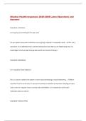
Karim, a new
Business
Studies graduate in Madrid, can earn €30 an hour. He must balance
earning enough to live comfortably with having free time to enjoy life.
His daily income (y) is determined by his wage (w) and hours worked
(h):
y=wh
Karim’s total income increases linearly with more hours worked, but
Figure 3.3: Karim’s income depends on his working hours.
he values both income for consumption and free time for leisure.
Therefore, his optimal work hours will reflect this balance.
His decision on work hours involves a trade-off: more consumption means less free time, and vice versa. His
preferences (a description of the relative values a person places on each possible outcome of a choice or decision
they have to make) can be illustrated using indifference curves, which show combinations of free time and
consumption that give him the same utility (a numerical indicator of the value that one places on an outcome).
These graphs are created by asking questions and plotting the combinations which give the same utility.
Key points about indifference curves:
1. Downward Sloping: More of one good requires less of the other to maintain the same utility.
2. Higher Curves = Higher Utility: More of both goods increases utility.
3. Smooth and Non-Crossing: Small changes in goods result in small utility changes, and curves don't intersect.
, 4. Marginal Rate of Substitution (MRS): Reflects how much consumption Karim is willing to sacrifice for more
free time; MRS decreases as he gets more free time (i.e. as you move to the right along an indifference
curve, it becomes flatter).
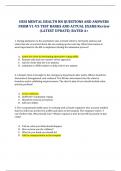
As you move up the vertical line at 15 hours of free time,
the indifference curves become steeper, indicating an
increase in the marginal rate of substitution (MRS). This
means that for a given amount of free time, Karim is
willing to sacrifice more consumption for an additional
hour of free time when his consumption is high
compared to when it is low. For instance, at point A
where his consumption is €540, the MRS is high (94): he
is willing to forgo €94 for an extra hour of free time,
illustrating the abundance of his consumption.
Conversely, if you keep consumption constant and
increase free time by moving right along the horizontal
line at €282, the MRS decreases along each indifference
Figure 3.5: The marginal rate of substitution.
curve. As free time becomes more abundant, Karim is
less willing to trade consumption for additional free
time.
It is important to note that while the MRS corresponds to the slope of the indifference curve, the MRS is expressed
as a positive number, whereas the slope of the indifference curve is negative. Thus, the MRS is the absolute value of
the slope.
Determining What is Feasible for Karim’s Indifference Curve:
Karim desires to maximize both his consumption spending and free time, but his choices are constrained by his wage
of €30 per hour. This creates a dilemma: increasing his free time reduces his potential consumption, highlighting the
opportunity cost of free time (what you lose when you choose one action rather than the next best alternative). His
budget constraint (an equation that represents all combinations of goods and services one could acquire that would
exactly exhaust one’s budgetary resources) is defined by his wage and the total hours he can work.
Budget Constraint Equation:
c = w(24-t)
Remember that if he works for ℎ hours at a wage 𝑤w, his income is 𝑦=𝑤ℎ. So, if he takes 𝑡 hours of free time, he will work
for (24−𝑡) hour per day, and his maximum level of consumption is 𝑐.
Figure 3.6 illustrates this budget constraint as a downward-
sloping line, showing feasible combinations of free time and
consumption. For instance, with 12 hours of free time, his
Figure 3.6: The budget maximum consumption is €360, not the €450 depicted at point
constraint and the feasible C, which is infeasible. Conversely, point D with 18 hours of free
set.
time and €70 of consumption, though feasible, is suboptimal
since he could increase consumption without sacrificing free
time.
Karim's feasible set (all of the combinations of goods or
outcomes that a decision-maker could choose, given the
economic, physical, or other constraints that they face) includes
all combinations on or below this budget constraint, with the
constraint itself forming the feasible frontier (the curve or line
made of points that defines the maximum feasible quantity of
one good for a given quantity of the other). The slope of this
Since the Industrial Revolution, technological progress has
dramatically increased wages, with American workers' real hourly
earnings rising sixfold in the 20th century. Average annual work
hours decreased by a third, allowing a fourfold increase in annual
earnings and a one-fifth increase in free time. Trends in income and
working hours vary by country, with higher-income countries
typically
enjoying
Figure 3.1: Annual hours of work and income (1870–2018). more free
time.
Differences arise due to individual preferences, job choices, and
legislation. While living standards have risen since 1870, some
countries prioritize higher consumption, others more free time.
Understanding Varying Working Hours Between Countries and
Over Time: Figure 3.2: Annual hours of free time per worker and income
(2020).
Goods are scarce if they are valued, and there is an opportunity
cost of acquiring more of them; this is a recurring problem in economics. Therefore, the following model will show
how people make choices when they cannot have all of everything that they want.
Karim, a new
Business
Studies graduate in Madrid, can earn €30 an hour. He must balance
earning enough to live comfortably with having free time to enjoy life.
His daily income (y) is determined by his wage (w) and hours worked
(h):
y=wh
Karim’s total income increases linearly with more hours worked, but
Figure 3.3: Karim’s income depends on his working hours.
he values both income for consumption and free time for leisure.
Therefore, his optimal work hours will reflect this balance.
His decision on work hours involves a trade-off: more consumption means less free time, and vice versa. His
preferences (a description of the relative values a person places on each possible outcome of a choice or decision
they have to make) can be illustrated using indifference curves, which show combinations of free time and
consumption that give him the same utility (a numerical indicator of the value that one places on an outcome).
These graphs are created by asking questions and plotting the combinations which give the same utility.
Key points about indifference curves:
1. Downward Sloping: More of one good requires less of the other to maintain the same utility.
2. Higher Curves = Higher Utility: More of both goods increases utility.
3. Smooth and Non-Crossing: Small changes in goods result in small utility changes, and curves don't intersect.
, 4. Marginal Rate of Substitution (MRS): Reflects how much consumption Karim is willing to sacrifice for more
free time; MRS decreases as he gets more free time (i.e. as you move to the right along an indifference
curve, it becomes flatter).
As you move up the vertical line at 15 hours of free time,
the indifference curves become steeper, indicating an
increase in the marginal rate of substitution (MRS). This
means that for a given amount of free time, Karim is
willing to sacrifice more consumption for an additional
hour of free time when his consumption is high
compared to when it is low. For instance, at point A
where his consumption is €540, the MRS is high (94): he
is willing to forgo €94 for an extra hour of free time,
illustrating the abundance of his consumption.
Conversely, if you keep consumption constant and
increase free time by moving right along the horizontal
line at €282, the MRS decreases along each indifference
Figure 3.5: The marginal rate of substitution.
curve. As free time becomes more abundant, Karim is
less willing to trade consumption for additional free
time.
It is important to note that while the MRS corresponds to the slope of the indifference curve, the MRS is expressed
as a positive number, whereas the slope of the indifference curve is negative. Thus, the MRS is the absolute value of
the slope.
Determining What is Feasible for Karim’s Indifference Curve:
Karim desires to maximize both his consumption spending and free time, but his choices are constrained by his wage
of €30 per hour. This creates a dilemma: increasing his free time reduces his potential consumption, highlighting the
opportunity cost of free time (what you lose when you choose one action rather than the next best alternative). His
budget constraint (an equation that represents all combinations of goods and services one could acquire that would
exactly exhaust one’s budgetary resources) is defined by his wage and the total hours he can work.
Budget Constraint Equation:
c = w(24-t)
Remember that if he works for ℎ hours at a wage 𝑤w, his income is 𝑦=𝑤ℎ. So, if he takes 𝑡 hours of free time, he will work
for (24−𝑡) hour per day, and his maximum level of consumption is 𝑐.
Figure 3.6 illustrates this budget constraint as a downward-
sloping line, showing feasible combinations of free time and
consumption. For instance, with 12 hours of free time, his
Figure 3.6: The budget maximum consumption is €360, not the €450 depicted at point
constraint and the feasible C, which is infeasible. Conversely, point D with 18 hours of free
set.
time and €70 of consumption, though feasible, is suboptimal
since he could increase consumption without sacrificing free
time.
Karim's feasible set (all of the combinations of goods or
outcomes that a decision-maker could choose, given the
economic, physical, or other constraints that they face) includes
all combinations on or below this budget constraint, with the
constraint itself forming the feasible frontier (the curve or line
made of points that defines the maximum feasible quantity of
one good for a given quantity of the other). The slope of this