Full file at http://testbank360.eu/solution -manual -fundamentals -of-fluid -mechanics -7th-edition -munson Munson
AComputational Fluid Dynamics A.1 Introduction Numerical methods using digital computers are, of course, commonly utilized to solve a wide variety of flow problems. As discussed in Chapter 6, although the differential equations that govern the flow of Newtonian fluids [the Navier –Stokes equations (Eq. 6.127)] were derived many years ago, there are few known analytical solutions to them. However, with the advent of highspeed digital computers it has become possible to obtain approximate numerical solutions to these (and other fluid mechanics) equations f or a wide variety of circumstances. Computational fluid dynamics (CFD) involves replacing the partial differential equations with discretized algebraic equations that approximate the partial differential equations. These equations are then numerically solved to obtain flow field values at the discrete points in space an d/or time. Since the Navier –Stokes equations are valid everywhere in the flow field of the fluid continuum, an analytical solution to these equations provides the solution for an infinite number of points in the flow. However, analytical solutions are available for only a limited number of simplified flow geometries. To overcome this limitation, the governing equations can be discretized and put in algebraic form for the computer to solve. The CFD simulation solves for the relev ant flow variables 726 Appendix A ■ Computational Fluid Dynamics Full file at http://testbank360.eu/solution -manual -fundamentals -of-fluid -mechanics -7th-edition -munson only at the discrete points, which make up the grid or mesh of the solution (discussed in more detail below). Interpolation schemes are used to obtain values at non -grid point locations. CFD can be thought of as a numerical experiment. In a typical fluids experiment, an experimental model is built, measurements of the flow interacting with that model are taken, and the results are analyzed. In CFD, the building of the model is replaced wit h the formulation of the governing equations and the development of the numerical algorithm. The process of obtaining measurements is replaced with running an algorithm on the computer to simulate the flow interaction. Of course, the analysis of results is common ground to both techniques. CFD can be classified as a subdiscipline to the study of fluid dynamics. However, it should be pointed out that a thorough coverage of CFD topics is well beyond the scope of this textbook. This appendix highlights some of the more important topics in CFD, but is only intended as a brief introduction. The topics include discretization of the governing equations, grid generation, boundary conditions, application of CFD, and some representative examples. A.2 Discretization The process of discretization involves developing a set of algebraic equations (based on discrete points in the flow domain) to be used in place of the partial differential equations. Of the various discretization techniques available for the numerical solution of the governing differe ntial equations, the following three types are most common: (1) the finite difference method, (2) the finite element (or finite volume) method, and (3) the boundary element method. In each of these methods, the continuous flow field (i.e., velocity or pressure as a function of space and time) is described in terms of discrete (rather than continuous) values at prescribed locations. Through this technique the differential equations are replaced by a set of algebraic equations th at can be solved on the computer. For the finite element (or finite volume ) method, the flow field is broken into a set of small fluid elements (usually triangular areas if the flow is two -dimensional, or small volume elements if the flow is three -dimensional). The conservation equations (i.e., conservation of mass, momentum, and energy) are written in an appropriate form for each element, and the set of resulting 725 Γi = strength of vortex on ■ Figure A.1 Panel method for ith panel flow past an airfoil. algebraic equations for the flow field is solved numerically. The number, size, and shape of elements are dictated in part by the particular flow geometry and flow conditions for the problem at hand. As the number of elements increases (as is necessary for flows with complex boundaries), the number of simultaneous algebraic equations that must be solved increases rapidly. Problems involving one million to ten million (or more) grid cells are not uncommon in today’s CFD community, particularly for complex th ree-dimensional geometries. Further information about this method can be found in Refs. 1 and 2. For the boundary element method , the boundary of the flow field (not the entire flow field as in the finite element method) is broken into discrete segments (Ref. 3) and appropriate singularities such as sources, sinks, doublets, and vortices are distributed on these boundary elements. The strengths and type of the singularities are chosen so that the appropriate boundary conditions of the flow are obtained on the boundary elements. For points in the flow field not on the boundary, the flow is calculated by adding the contributions from the various singularities on the boundary. Although the details of this method are rather mathematically sophisticated, it may (depending on VA.1 Pouring a liquid i i th Γ U i Γ i Γ
AComputational Fluid Dynamics A.1 Introduction Numerical methods using digital computers are, of course, commonly utilized to solve a wide variety of flow problems. As discussed in Chapter 6, although the differential equations that govern the flow of Newtonian fluids [the Navier –Stokes equations (Eq. 6.127)] were derived many years ago, there are few known analytical solutions to them. However, with the advent of highspeed digital computers it has become possible to obtain approximate numerical solutions to these (and other fluid mechanics) equations f or a wide variety of circumstances. Computational fluid dynamics (CFD) involves replacing the partial differential equations with discretized algebraic equations that approximate the partial differential equations. These equations are then numerically solved to obtain flow field values at the discrete points in space an d/or time. Since the Navier –Stokes equations are valid everywhere in the flow field of the fluid continuum, an analytical solution to these equations provides the solution for an infinite number of points in the flow. However, analytical solutions are available for only a limited number of simplified flow geometries. To overcome this limitation, the governing equations can be discretized and put in algebraic form for the computer to solve. The CFD simulation solves for the relev ant flow variables 726 Appendix A ■ Computational Fluid Dynamics Full file at http://testbank360.eu/solution -manual -fundamentals -of-fluid -mechanics -7th-edition -munson only at the discrete points, which make up the grid or mesh of the solution (discussed in more detail below). Interpolation schemes are used to obtain values at non -grid point locations. CFD can be thought of as a numerical experiment. In a typical fluids experiment, an experimental model is built, measurements of the flow interacting with that model are taken, and the results are analyzed. In CFD, the building of the model is replaced wit h the formulation of the governing equations and the development of the numerical algorithm. The process of obtaining measurements is replaced with running an algorithm on the computer to simulate the flow interaction. Of course, the analysis of results is common ground to both techniques. CFD can be classified as a subdiscipline to the study of fluid dynamics. However, it should be pointed out that a thorough coverage of CFD topics is well beyond the scope of this textbook. This appendix highlights some of the more important topics in CFD, but is only intended as a brief introduction. The topics include discretization of the governing equations, grid generation, boundary conditions, application of CFD, and some representative examples. A.2 Discretization The process of discretization involves developing a set of algebraic equations (based on discrete points in the flow domain) to be used in place of the partial differential equations. Of the various discretization techniques available for the numerical solution of the governing differe ntial equations, the following three types are most common: (1) the finite difference method, (2) the finite element (or finite volume) method, and (3) the boundary element method. In each of these methods, the continuous flow field (i.e., velocity or pressure as a function of space and time) is described in terms of discrete (rather than continuous) values at prescribed locations. Through this technique the differential equations are replaced by a set of algebraic equations th at can be solved on the computer. For the finite element (or finite volume ) method, the flow field is broken into a set of small fluid elements (usually triangular areas if the flow is two -dimensional, or small volume elements if the flow is three -dimensional). The conservation equations (i.e., conservation of mass, momentum, and energy) are written in an appropriate form for each element, and the set of resulting 725 Γi = strength of vortex on ■ Figure A.1 Panel method for ith panel flow past an airfoil. algebraic equations for the flow field is solved numerically. The number, size, and shape of elements are dictated in part by the particular flow geometry and flow conditions for the problem at hand. As the number of elements increases (as is necessary for flows with complex boundaries), the number of simultaneous algebraic equations that must be solved increases rapidly. Problems involving one million to ten million (or more) grid cells are not uncommon in today’s CFD community, particularly for complex th ree-dimensional geometries. Further information about this method can be found in Refs. 1 and 2. For the boundary element method , the boundary of the flow field (not the entire flow field as in the finite element method) is broken into discrete segments (Ref. 3) and appropriate singularities such as sources, sinks, doublets, and vortices are distributed on these boundary elements. The strengths and type of the singularities are chosen so that the appropriate boundary conditions of the flow are obtained on the boundary elements. For points in the flow field not on the boundary, the flow is calculated by adding the contributions from the various singularities on the boundary. Although the details of this method are rather mathematically sophisticated, it may (depending on VA.1 Pouring a liquid i i th Γ U i Γ i Γ