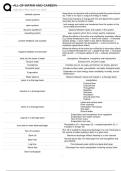
CAQ SPSS
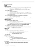
Principal Component Analysis (PCA)
Analyze → Dimension Reduction → Factor. Drag all variables into the window
Enable following options:
- KMO and Bartlett’s test of sphericity in Descriptive.
- Extraction menu: Principal Components and Scree Plot
- Options menu → Sorted by Size and Suppress Small Coefficients (value below 0.3)
Example:
FACTOR /VARIABLES v225 v226 v227 v228 v229 v230 v231 v232 v233 v234 v235 v236 v237 v238 v239 v240 v241 v242
/MISSING LISTWISE /ANALYSIS v225 v226 v227 v228 v229 v230 v231 v232 v233 v234 v235 v236 v237 v238 v239 v240 v241 v242
/PRINT INITIAL KMO EXTRACTION
/FORMAT SORT BLANK(.30)
/PLOT EIGEN
/CRITERIA MINEIGEN(1) ITERATE(25)
/EXTRACTION PC /ROTATION NOROTATE
/METHOD=CORRELATION.
Assumptions of PCA
Two tests that indicate suitability of our date for running PCA:
- KMO: A high value (close to 1.0) indicates that it is reasonable to run a PCA (the
higher the value, the better). A rule of thumb is that this value should be equal to at
least 0.6.
- Bartlett’s test of sphericity: When significant (e.g. p-value < 0.05), it indicates that
it is reasonable to run a PCA.
Communalities = The communality of an item is the amount of variance in that item that is
explained by all components. It is a measure of how well the components explain people’s
answers to that item.
→ You can find this in table communalities → column extraction
Eigenvalues = The eigenvalue of a component indicates how much variance is explained by
that component. The eigenvalue is equal to
the sum of the explained variance of all
items on the relevant component.
→ you can find this in table Total
Variance Explained → Column total
Component loading = component loading
represents the correlation between an item and a component. For example, if item 1 has a
component loading of 0.50 on component 1, this means that they correlate to +0.50
→ You can find this in table Component Matrix
Choosing the number of components for PCA rule of thumb
- Kaiser Guttman (Kaiser’s rule): the number of components that should be chosen
is equal to the number of components with an eigenvalue >1.
- Based on scree plot: elbow point; ook for an abrupt change in the slope, known as
the elbow point, and choose the number of principal components before that point.