Solution Manual For:
Introduction to Linear Optimization
by Dimitris Bertsimas & John N. Tsitsiklis
John L. Weatherwax∗
November 22, 2007
Introduction
Acknowledgements
Special thanks to Dave Monet for helping find and correct various typos in these solutions.
Chapter 1 (Introduction)
Exercise 1.1
Since f (·) is convex we have that
f (λx + (1 − λ)y) ≤ λf (x) + (1 − λ)f (y) . (1)
Since f (·) is concave we also have that
f (λx + (1 − λ)y) ≥ λf (x) + (1 − λ)f (y) . (2)
Combining these two expressions we have that f must satisfy each with equality or
f (λx + (1 − λ)y) = λf (x) + (1 − λ)f (y) . (3)
This implies that f must be linear and the expression given in the book holds.
∗
1
,Exercise 1.2
Part (a): We are told that fi is convex so we have that
fi (λx + (1 − λ)y) ≤ λfi (x) + (1 − λ)fi (y) , (4)
for every i. For our function f (·) we have that
m
X
f (λx + (1 − λ)y) = fi (λx + (1 − λ)y) (5)
i=1
m
X
≤ λfi (x) + (1 − λ)fi (y) (6)
i=1
Xm m
X
= λ fi (x) + (1 − λ) fi (y) (7)
i=1 i=1
= λf (x) + (1 − λ)f (y) (8)
and thus f (·) is convex.
Part (b): The definition of a piecewise linear convex function fi is that is has a represen-
tation given by
fi (x) = Maxj=1,2,...,m (c′j x + dj ) . (9)
So our f (·) function is
n
X
f (x) = Maxj=1,2,...,m (c′j x + dj ) . (10)
i=1
Now for each of the fi (x) piecewise linear convex functions i ∈ 1, 2, 3, . . . , n we are adding
up in the definition of f (·) we will assume that function fi (x) has mi affine/linear functions
to maximize over. Now select a new set of affine values (c̃j , d˜j ) formed by summing elements
from each of the 1, 2, 3, . . . , n sets of coefficients from the individual fi . Each pair of (c̃j , d˜j )
is obtained by summing one of the (cj , dj ) pairs from each of the n sets. The number of
such coefficients can be determined as follows. We have m1 choices to make when selecting
(cj , dj ) from the first piecewise linear convex function, m2 choices for the second piecewise
linear convex function, and so on giving a total of m1 m2 m3 · · · mn total possible sums each
producing a single pair (c̃j , d˜j ). Thus we can see that f (·) can be written as
f (x) = Maxj=1,2,3,...,Qnl=1 ml c̃′j x + d˜j , (11)
since one of the (c̃j , d˜j ) will produce the global maximum. This shows that f (·) can be
written as a piecewise linear convex function.
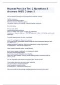
Exercise 1.3 (minimizing a linear plus linear convex constraint)
We desire to convert the problem min(c′ x + f (x)) subject to the linear constraint Ax ≥ b,
with f (x) given as in the picture to the standard form for linear programming. The f (·)
, given in the picture can be represented as
−ξ + 1 ξ<1
f (ξ) = 0 1<ξ<2 (12)
2(ξ − 2) ξ > 2,
but it is better to recognize this f (·) as a piecewise linear convex function given by the
maximum of three individual linear functions as
f (ξ) = max (−ξ + 1, 0, 2ξ − 4) (13)
Defining z ≡ max (−ξ + 1, 0, 2ξ − 4) we see that or original problem of minimizing over the
term f (x) is equivalent to minimizing over z. This in tern is equivalent to requiring that z
be the smallest value that satisfies
z ≥ −ξ + 1 (14)
z ≥ 0 (15)
z ≥ 2ξ − 4 . (16)
With this definition, our original problem is equivalent to
Minimize (c′ x + z) (17)
subject to the following constraints
Ax ≥ b (18)
z ≥ −d′ x + 1 (19)
z ≥ 0 (20)
z ≥ 2d′ x + 4 (21)
where the variables to minimize over are (x, z). Converting to standard form we have the
problem
Minimize(c′ x + z) (22)
subject to
Ax ≥ b (23)
′
dx+z ≥ 1 (24)
z ≥ 0 (25)
′
−2d x + z ≥ 4 (26)
Exercise 1.4
Our problem is
Minimize(2x1 + 3|x2 − 10|) (27)
subject to
|x1 + 2| + |x2 | ≤ 5 . (28)
Introduction to Linear Optimization
by Dimitris Bertsimas & John N. Tsitsiklis
John L. Weatherwax∗
November 22, 2007
Introduction
Acknowledgements
Special thanks to Dave Monet for helping find and correct various typos in these solutions.
Chapter 1 (Introduction)
Exercise 1.1
Since f (·) is convex we have that
f (λx + (1 − λ)y) ≤ λf (x) + (1 − λ)f (y) . (1)
Since f (·) is concave we also have that
f (λx + (1 − λ)y) ≥ λf (x) + (1 − λ)f (y) . (2)
Combining these two expressions we have that f must satisfy each with equality or
f (λx + (1 − λ)y) = λf (x) + (1 − λ)f (y) . (3)
This implies that f must be linear and the expression given in the book holds.
∗
1
,Exercise 1.2
Part (a): We are told that fi is convex so we have that
fi (λx + (1 − λ)y) ≤ λfi (x) + (1 − λ)fi (y) , (4)
for every i. For our function f (·) we have that
m
X
f (λx + (1 − λ)y) = fi (λx + (1 − λ)y) (5)
i=1
m
X
≤ λfi (x) + (1 − λ)fi (y) (6)
i=1
Xm m
X
= λ fi (x) + (1 − λ) fi (y) (7)
i=1 i=1
= λf (x) + (1 − λ)f (y) (8)
and thus f (·) is convex.
Part (b): The definition of a piecewise linear convex function fi is that is has a represen-
tation given by
fi (x) = Maxj=1,2,...,m (c′j x + dj ) . (9)
So our f (·) function is
n
X
f (x) = Maxj=1,2,...,m (c′j x + dj ) . (10)
i=1
Now for each of the fi (x) piecewise linear convex functions i ∈ 1, 2, 3, . . . , n we are adding
up in the definition of f (·) we will assume that function fi (x) has mi affine/linear functions
to maximize over. Now select a new set of affine values (c̃j , d˜j ) formed by summing elements
from each of the 1, 2, 3, . . . , n sets of coefficients from the individual fi . Each pair of (c̃j , d˜j )
is obtained by summing one of the (cj , dj ) pairs from each of the n sets. The number of
such coefficients can be determined as follows. We have m1 choices to make when selecting
(cj , dj ) from the first piecewise linear convex function, m2 choices for the second piecewise
linear convex function, and so on giving a total of m1 m2 m3 · · · mn total possible sums each
producing a single pair (c̃j , d˜j ). Thus we can see that f (·) can be written as
f (x) = Maxj=1,2,3,...,Qnl=1 ml c̃′j x + d˜j , (11)
since one of the (c̃j , d˜j ) will produce the global maximum. This shows that f (·) can be
written as a piecewise linear convex function.
Exercise 1.3 (minimizing a linear plus linear convex constraint)
We desire to convert the problem min(c′ x + f (x)) subject to the linear constraint Ax ≥ b,
with f (x) given as in the picture to the standard form for linear programming. The f (·)
, given in the picture can be represented as
−ξ + 1 ξ<1
f (ξ) = 0 1<ξ<2 (12)
2(ξ − 2) ξ > 2,
but it is better to recognize this f (·) as a piecewise linear convex function given by the
maximum of three individual linear functions as
f (ξ) = max (−ξ + 1, 0, 2ξ − 4) (13)
Defining z ≡ max (−ξ + 1, 0, 2ξ − 4) we see that or original problem of minimizing over the
term f (x) is equivalent to minimizing over z. This in tern is equivalent to requiring that z
be the smallest value that satisfies
z ≥ −ξ + 1 (14)
z ≥ 0 (15)
z ≥ 2ξ − 4 . (16)
With this definition, our original problem is equivalent to
Minimize (c′ x + z) (17)
subject to the following constraints
Ax ≥ b (18)
z ≥ −d′ x + 1 (19)
z ≥ 0 (20)
z ≥ 2d′ x + 4 (21)
where the variables to minimize over are (x, z). Converting to standard form we have the
problem
Minimize(c′ x + z) (22)
subject to
Ax ≥ b (23)
′
dx+z ≥ 1 (24)
z ≥ 0 (25)
′
−2d x + z ≥ 4 (26)
Exercise 1.4
Our problem is
Minimize(2x1 + 3|x2 − 10|) (27)
subject to
|x1 + 2| + |x2 | ≤ 5 . (28)