Statistiek Summary chapter 5-19
Lecture: Statistics for pre-master. Year: 2017.
Inhoud
Chapter 5 ....................................................................................................................................................... 2
Chapter 6 ....................................................................................................................................................... 8
Chapter 7 ..................................................................................................................................................... 10
Chapter 8 ..................................................................................................................................................... 12
Chapter 9 ..................................................................................................................................................... 17
Chapter 10 ................................................................................................................................................... 18
Chapter 11 ................................................................................................................................................... 21
Chapter 12 ................................................................................................................................................... 24
Chapter 13 ................................................................................................................................................... 26
Chapter 14 ................................................................................................................................................... 27
Chapter 15 ................................................................................................................................................... 28
Chapter 16 ................................................................................................................................................... 32
Chapter 17 ................................................................................................................................................... 36
1
,Chapter 5
Wetenschappelijke benamingen:
(𝒙𝟏 , 𝒚𝟏 ), (𝒙𝟐 𝒚𝟐 ), … … , (𝒙𝑵 𝒚𝑵 ): population dataset
(𝒙𝟏 , 𝒚𝟏 ), (𝒙𝟐 𝒚𝟐 ), … … , (𝒙𝒏 𝒚𝒏 ): sample dataset.
𝝈𝒙,𝒚 : population covariance
𝒔𝒙,𝒚 : sample covariance
𝝈𝟐𝒙 : population variance
𝒔𝟐𝒙 : sample variance
𝝆 (𝒐𝒓 𝝆𝑿,𝒀 ): population correlation coefficient
𝒓 (𝒐𝒓 𝒓𝑿,𝒀 ): sample correlation coefficient
𝒃𝟎 𝒂𝒏𝒅 𝒃𝟏 : sample regression coefficients.
𝜷𝟎 𝒂𝒏𝒅 𝜷𝟏 : population regression coefficients.
𝛃𝟎 𝐨𝐫 𝐛𝟎: intercept
𝛃𝟏 𝐨𝐫 𝐛𝟏: slope
𝐲̂: prediction line
In this chapter one of the following three primary objectives is aimed at (depending on problem of
interest)
1. Positioning the population elements with respect to each other by comparing the datasets of
two variables.
2. Studying the combined relationship of X and Y with time(if the datasets are time series)
3. Studying the dependence of the data of one variable on the data of the other variable.
The most attention will be paid at situation 3.
5.1 Scatter plot, covariance and correlation
The dependent variable is denoted as Y and de independent variable is denoted as X. Research is aimed
at finding out whether Y is related to X. For example is the GDP(Y) related to the inflation rate(X)?
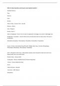
To get an impression of the way the y data depend on the
corresponding x data, one constructs a scatter plot of y on x (=one
puts the n pairs of data into a 2D system of axes, where the horizontal
x-axis refers to the independent variable and the vertical y-axis refers
to the dependent variable.) See image ->
In the x, y plane, a cloud of dots results, this is called a population
cloud or a sample cloud.
Y and x are positively linearly related when there is an increasing
straight line, y and x are negatively linearly related if there is a
decreasing straight line.
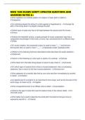
X and y have a quadratic relationship when the curve is a mountain-
shaped parabolic (first increases and then declines). See image->
Focus in this chapter will be on the linear relationship between two
variables.
Population dataset: (𝑥1 , 𝑦1 ), (𝑥2 𝑦2 ), … … , (𝑥𝑁 𝑦𝑁 )
Sample dataset: (𝑥1 , 𝑦1 ), (𝑥2 𝑦2 ), … … , (𝑥𝑛 𝑦𝑛 )
We want the so called measures of association, that measures the strength
of the linear relationship.
2
,Population covariance (𝜎𝑥,𝑦 ):
N
1
𝜎𝑥,𝑦 = ∑(xi − μy )
N
i=1
Sample covariance (𝑠𝑥,𝑦 ):
N
1
𝑠𝑥,𝑦 = ∑(xi − x̅) (yi − y̅)
n−1
i=1
𝑠𝑥,𝑦 is often used as estimate of the unknown 𝜎𝑥,𝑦 .
Population variance:
𝜎𝑥,𝑥 = 𝜎𝑥2
Sample variance:
𝑠𝑥,𝑥 = 𝑠𝑥2
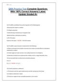
For example:
In this example the 𝑠𝑥2 , 𝑠𝑦2 𝑎𝑛𝑑 𝑠𝑥,𝑦 can
be calculated.
1 46
𝑠𝑥2 = × 46 =
(13 − 1) (13 − 1)
75.08
𝑠𝑥2 =
(13 − 1)
26
𝑠𝑥,𝑦 =
(13 − 1)
The statistic correlation coefficient is a measure of linear relationship that does not have the following
disadvantages that the covariance has:
The covariance is not immediately suitable to measure the strength of a linear relationship (it
does not reflect whether it is a strong or weak linear relationship, because a reference point is
missing)
The covariance depends on the dimensions (the unit in which the variables are measured), for
example the unit 106 euro.
The sample correlation coefficient r (or 𝑟𝑋,𝑌 ) is defined as the ratio of the sample covariance and the
product of the two sample standard deviations.
𝑠𝑋,𝑌
𝑟 = 𝑟𝑋,𝑌 =
𝑠𝑋 𝑠𝑌
The population correlation coefficient 𝜌 (𝑜𝑟 𝜌𝑋,𝑌 ) is defined as the ratio of the population covariance
and the product of the two population standard deviations.
3
, 𝜎𝑋,𝑌
𝜌 = 𝜌𝑋,𝑌 =
𝜎𝑋 𝜎𝑌
The standard deviations can be calculated by √𝑠𝑥2 or √𝜎𝑥2 (de wortel nemen van de variantie).
Properties of correlation coefficients
Can never be larger than +1 or smaller than -1.
+1 means that all pairs of x and y fall precisely on one increasing straight line.
-1 means that all pairs of x and y fall precisely on one decreasing straight line.
0 Means that x and y are uncorrelated.
Correlation only measures linear dependence between Y and X, there still can exist another
relationship such as the quadratic one.
5.2 Regression line
Regression of Y on X: how Y depends on X.
Least-squares method: determines the constants a and b such that the sum of the squared deviations is
as small as possible. For example y = bo + b1 x. To determine bo and b1 the least-squares method is
used.
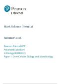
The vertical deviations, also called errors or residuals are (see arrow on image below):
𝑦1 − (𝑏𝑜 + 𝑏1 𝑥1 ), 𝑦2 − (𝑏𝑜 + 𝑏1 𝑥2 ), … . , (𝑏𝑜 + 𝑏1 𝑥𝑛 )
The sum of these squared deviations, have to be minimal and that is what the least-squares method
calculates.
𝑛
∑(𝑦𝑖 − (𝑎 + 𝑏𝑥𝑖 ))2
𝑖=1
This LS method yields the optimal constants denoted by 𝑏0 𝑎𝑛𝑑 𝑏1 and are called sample regression
coefficients. The constants denoted by 𝛽0 𝑎𝑛𝑑 𝛽1 are called population regression coefficients.
sX,Y
b1 = 2 and b0 = y̅ − b1 x̅
sX
σX,Y
β1 = 2 and β0 = μy − β1 μx
σX
Sample regression line
4
Lecture: Statistics for pre-master. Year: 2017.
Inhoud
Chapter 5 ....................................................................................................................................................... 2
Chapter 6 ....................................................................................................................................................... 8
Chapter 7 ..................................................................................................................................................... 10
Chapter 8 ..................................................................................................................................................... 12
Chapter 9 ..................................................................................................................................................... 17
Chapter 10 ................................................................................................................................................... 18
Chapter 11 ................................................................................................................................................... 21
Chapter 12 ................................................................................................................................................... 24
Chapter 13 ................................................................................................................................................... 26
Chapter 14 ................................................................................................................................................... 27
Chapter 15 ................................................................................................................................................... 28
Chapter 16 ................................................................................................................................................... 32
Chapter 17 ................................................................................................................................................... 36
1
,Chapter 5
Wetenschappelijke benamingen:
(𝒙𝟏 , 𝒚𝟏 ), (𝒙𝟐 𝒚𝟐 ), … … , (𝒙𝑵 𝒚𝑵 ): population dataset
(𝒙𝟏 , 𝒚𝟏 ), (𝒙𝟐 𝒚𝟐 ), … … , (𝒙𝒏 𝒚𝒏 ): sample dataset.
𝝈𝒙,𝒚 : population covariance
𝒔𝒙,𝒚 : sample covariance
𝝈𝟐𝒙 : population variance
𝒔𝟐𝒙 : sample variance
𝝆 (𝒐𝒓 𝝆𝑿,𝒀 ): population correlation coefficient
𝒓 (𝒐𝒓 𝒓𝑿,𝒀 ): sample correlation coefficient
𝒃𝟎 𝒂𝒏𝒅 𝒃𝟏 : sample regression coefficients.
𝜷𝟎 𝒂𝒏𝒅 𝜷𝟏 : population regression coefficients.
𝛃𝟎 𝐨𝐫 𝐛𝟎: intercept
𝛃𝟏 𝐨𝐫 𝐛𝟏: slope
𝐲̂: prediction line
In this chapter one of the following three primary objectives is aimed at (depending on problem of
interest)
1. Positioning the population elements with respect to each other by comparing the datasets of
two variables.
2. Studying the combined relationship of X and Y with time(if the datasets are time series)
3. Studying the dependence of the data of one variable on the data of the other variable.
The most attention will be paid at situation 3.
5.1 Scatter plot, covariance and correlation
The dependent variable is denoted as Y and de independent variable is denoted as X. Research is aimed
at finding out whether Y is related to X. For example is the GDP(Y) related to the inflation rate(X)?
To get an impression of the way the y data depend on the
corresponding x data, one constructs a scatter plot of y on x (=one
puts the n pairs of data into a 2D system of axes, where the horizontal
x-axis refers to the independent variable and the vertical y-axis refers
to the dependent variable.) See image ->
In the x, y plane, a cloud of dots results, this is called a population
cloud or a sample cloud.
Y and x are positively linearly related when there is an increasing
straight line, y and x are negatively linearly related if there is a
decreasing straight line.
X and y have a quadratic relationship when the curve is a mountain-
shaped parabolic (first increases and then declines). See image->
Focus in this chapter will be on the linear relationship between two
variables.
Population dataset: (𝑥1 , 𝑦1 ), (𝑥2 𝑦2 ), … … , (𝑥𝑁 𝑦𝑁 )
Sample dataset: (𝑥1 , 𝑦1 ), (𝑥2 𝑦2 ), … … , (𝑥𝑛 𝑦𝑛 )
We want the so called measures of association, that measures the strength
of the linear relationship.
2
,Population covariance (𝜎𝑥,𝑦 ):
N
1
𝜎𝑥,𝑦 = ∑(xi − μy )
N
i=1
Sample covariance (𝑠𝑥,𝑦 ):
N
1
𝑠𝑥,𝑦 = ∑(xi − x̅) (yi − y̅)
n−1
i=1
𝑠𝑥,𝑦 is often used as estimate of the unknown 𝜎𝑥,𝑦 .
Population variance:
𝜎𝑥,𝑥 = 𝜎𝑥2
Sample variance:
𝑠𝑥,𝑥 = 𝑠𝑥2
For example:
In this example the 𝑠𝑥2 , 𝑠𝑦2 𝑎𝑛𝑑 𝑠𝑥,𝑦 can
be calculated.
1 46
𝑠𝑥2 = × 46 =
(13 − 1) (13 − 1)
75.08
𝑠𝑥2 =
(13 − 1)
26
𝑠𝑥,𝑦 =
(13 − 1)
The statistic correlation coefficient is a measure of linear relationship that does not have the following
disadvantages that the covariance has:
The covariance is not immediately suitable to measure the strength of a linear relationship (it
does not reflect whether it is a strong or weak linear relationship, because a reference point is
missing)
The covariance depends on the dimensions (the unit in which the variables are measured), for
example the unit 106 euro.
The sample correlation coefficient r (or 𝑟𝑋,𝑌 ) is defined as the ratio of the sample covariance and the
product of the two sample standard deviations.
𝑠𝑋,𝑌
𝑟 = 𝑟𝑋,𝑌 =
𝑠𝑋 𝑠𝑌
The population correlation coefficient 𝜌 (𝑜𝑟 𝜌𝑋,𝑌 ) is defined as the ratio of the population covariance
and the product of the two population standard deviations.
3
, 𝜎𝑋,𝑌
𝜌 = 𝜌𝑋,𝑌 =
𝜎𝑋 𝜎𝑌
The standard deviations can be calculated by √𝑠𝑥2 or √𝜎𝑥2 (de wortel nemen van de variantie).
Properties of correlation coefficients
Can never be larger than +1 or smaller than -1.
+1 means that all pairs of x and y fall precisely on one increasing straight line.
-1 means that all pairs of x and y fall precisely on one decreasing straight line.
0 Means that x and y are uncorrelated.
Correlation only measures linear dependence between Y and X, there still can exist another
relationship such as the quadratic one.
5.2 Regression line
Regression of Y on X: how Y depends on X.
Least-squares method: determines the constants a and b such that the sum of the squared deviations is
as small as possible. For example y = bo + b1 x. To determine bo and b1 the least-squares method is
used.
The vertical deviations, also called errors or residuals are (see arrow on image below):
𝑦1 − (𝑏𝑜 + 𝑏1 𝑥1 ), 𝑦2 − (𝑏𝑜 + 𝑏1 𝑥2 ), … . , (𝑏𝑜 + 𝑏1 𝑥𝑛 )
The sum of these squared deviations, have to be minimal and that is what the least-squares method
calculates.
𝑛
∑(𝑦𝑖 − (𝑎 + 𝑏𝑥𝑖 ))2
𝑖=1
This LS method yields the optimal constants denoted by 𝑏0 𝑎𝑛𝑑 𝑏1 and are called sample regression
coefficients. The constants denoted by 𝛽0 𝑎𝑛𝑑 𝛽1 are called population regression coefficients.
sX,Y
b1 = 2 and b0 = y̅ − b1 x̅
sX
σX,Y
β1 = 2 and β0 = μy − β1 μx
σX
Sample regression line
4