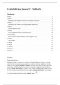
Contents
Week 0........................................................................................................................................1
Lecture 1.....................................................................................................................................2
knowledge clip: Confidence intervals and sampling fluctuations..........................................6
Lecture 2.....................................................................................................................................8
Knowledge clip: statistical power and multiple comparisons..............................................12
Lecture 3...................................................................................................................................13
Bayesian statistics (clip).......................................................................................................19
Lecture 4...................................................................................................................................19
Clip: assumptions multiple regression analysis....................................................................19
Lecture 5 and 6.........................................................................................................................22
Clip: correlation between bitterness and psychopathic traits...............................................30
Lecture 7...................................................................................................................................30
Adjusted R^2........................................................................................................................36
Lecture 8...................................................................................................................................37
Lecture 9...................................................................................................................................43
Lecture 10.................................................................................................................................48
Lecture 11v...............................................................................................................................55
Lecture 12.................................................................................................................................61
Week 0
Recap from Statistics 1
Hypothesis testing: we want to draw conclusions about a population. However, it usually
cannot be done to study an entire population so we draw a (random) sample and with this
sample, we can calculate descriptive statistics such as the mean. However, the value of the
sample mean will differ slightly every time you draw a new sample from the population >
these are sample fluctuations. If we draw a huge amount of samples and calculate the mean
for each one and put these in a distribution, we get a sampling distribution > the standard
error of this sampling distribution is the standard error ( )
,We use hypothesis testing for inferential statistics = drawing inferences about the
population based on the sample. > steps are:
1. We create a null hypothesis which shows what would happen if there would be no
change and an alternative hypothesis which shows what would happen if there is a
change (directional: higher or lower or non-directional: different). We assume that the
null hypothesis is true until proven otherwise
2. We calculate the standard error which we need to calculate a test-statistic > the 2
most common test-statistics (we use) are z-scores and t-scores.
3. We set a significance level (alpha), usually 0.05 so we can decide the area of
rejection. If the calculated test statistic falls outside of the area of rejection, we
cannot reject H0. If the test-statistic falls inside the area of rejection, we can reject H0.
4. We make a decision on whether our calculated test-statistic (z or t score) fall inside or
outside our previously determined boundaries (alpha level)
a. So, in an SPSS table, we look at the p-value = the probability of obtaining a
t-value equal to or higher than 1.783 (the t-value the SPSS table gives) AND
the probability of obtaining a t-value equal to or lower than -1.783 when the
null hypothesis is true = the probability of obtaining a test result (t value or z
value) at least as extreme as the result actually observed, if H0 is correct (the )
b. If the p-value (generated by the SPSS table) is larger than the alpha level (we
have previously set), we cannot reject H0
c. If the p-value (generated by the SPSS table) is smaller than the alpha level, we
reject H0
Lecture 1
Population = a set of scores for the entire population of interest
Sample = small sub-set of the population
- Representative sample = if the cases in the sample have characteristics similar to
those of the population (e.g. nation-state where 10% in Hispanic, 10% is Asian and
80% is Caucasian, you would have your sample be distributed in the same way)
- Sampling designs (important for this course):
o Simple random sampling = every member in the population has an equal
chance to be sampled
o Stratified sampling = the population is divided into strata (e.g. based on age;
12-18, 18-25 etc) and within each stratum, a random sample is drawn
o Convenience sampling = asking people who are readily available (friends,
family etc)
Can result into a problem as the sample may not be representative of
the population
- Descriptive statistics: summarizing data, giving information about the sample data
o Measures of central tendency
Mean = average
Median = one in the middle
Mode = one that occurs the most often
o Measures of dispersion
, Variance
Standard deviation
o E.g. do women perform better on the exam than men? > look at mean for both
groups, compare means > conclusion
Inferential statistics = making generalizations about the population, using the information
from the sample
- 2 main procedures
o Null hypothesis significance testing (see week 0)
o Confidence interval estimation (see below)
- Sampling error (see also above) = different samples drawn from the same population
will differ slightly in their sample means. This variation between sample means is
expressed as the sampling error (or: the standard deviation of the sample means)
(written as σm)
o The distribution of sample means is called the sampling distribution of M
and has:
A mean of µ
And a standard error of σm (in the population)
Data / data set = information (usually numerical) about multiple cases and / or multiple
variables
- Variable = characteristic that differs or varies across subjects or cases (e.g.
height, salary, heart rate)
o Categorical variables = identify groups or categories for each case (e.g.
gender, marital status, education level)
Always nominal variables = there is no scale on how you score on
the variable. It is either one or the other (e.g. 1 = female, 2 = male)
> the numbers that we use in nominal variables are purely random,
they only have a meaning because we assign the meaning to them
(so you can also say 1 = male and 2 = female, it does not matter for
the analysis)
You cannot compare the numbers that we assign to the nominal
variable in terms of ‘greater than’ or ‘less than’ > we do not use
mathematical operations on these numbers (+. -, *) > so we also
cannot calculate the mean for the numbers > we can only say that
they are different
o Quantitative variable = indicate how much of some characteristic or
behaviour each case or person has (e.g. blood pressure)
Because the numerical scores have actual meaning, we can
compare them in less and more (e.g. person A has a higher blood
pressure than person B)
o Ordinal variables =
- Subjects / cases = the entities or observational units studied (e.g. a person, an
organization, a nation-state, a geographical location)
Analysis = statistical techniques (to interpret the data)
- Problems in interpreting results
o Describing an association as causal when there is no evidence to support
this
, o Overgeneralizing the results to populations and situations that are not
similar to those included in the study
o Misunderstanding or minimizing the limitations of the design and analysis
- Problems in significance testing
o P-hacking = researchers will alter the data set (drop outliers, change from a
2-tailed test to a 1-tailed test) to achieve p < 0.05.
o A highly significant p-value does not mean that there is a strong effect or
practical importance
Statistical significance = when results are unlikely to arise by just
chance > never use the phrase ‘highly significant’ to describe
research outcomes with small p values
Clinical / practical significance = what it actually means and
contributes to every-day life
Experimental research design = two or more groups of cases where each group is exposed
to a different type of treatment / different amounts of treatment (independent variable) and
see how that influences the dent variable (thing you want to measure)
- Experimental control
o Random assignment to conditions = each subject has an equal chance of
being placed in either group
Unlucky randomization = even when random assignment has
been applied, the groups end up being different in some way just
by chance
o Control the type and amount of treatment
o Control over situational factors / extraneous variables: you want to keep
all other things equal (e.g. time of day, the mood of the researcher)
Correlational study = measures 2 or more variables that are believed to be meaningfully
related and the researcher does not introduce a treatment of intervention
Quasi-experimental: compare group outcomes but lack the full controls that are needed for
an experiment (mainly random assignment)
This course is (obviously) about correlational research.
Pearson’s correlation coefficient

