REVISION
Term 1
The market
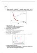
- Market equilibrium = intersection of downward sloping demand curve &
(vertical short-run) supply curve at equilibrium price & quantity clearing market
Willingness to pay
pay pe / more than
pe
- Case of low price: QD > QS
o Quantity demanded (QD) > quantity supplied (QS)
o Price adjustment through increase to pe
Market eventually coming up to QD = QS
- Case of high price: QD < QS
o Quantity demanded (QD) < quantity supplied (QS)
o Price adjustment through decrease to pe
Market eventually coming down to QD = QS
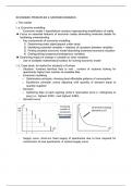
- Increase in quantity supplied
o Increase QS shift supply curve to new quantity supplied decrease of pe
- Increase in income of consumers
o Increase in consumers’ willingness to pay upward shift of demand curve
to new reservation prices’ levels increase of pe
, - Increase in number of consumers with identical distribution preferences
o Increase in QD rightward shift of demand curve increase of pe
- Criterion Pareto efficiency: examining plausibility/desirability of other modes
of allocation
o Desirable outcome: ≠ other way allocating goods such some people better
off & no one made less well off
Budget constraint
- Consumption bundle x = (x1, x2) with vector of commodity prices p = (p1, p2)
Consumption bundle x affordable at vector of prices p if
x1p1 + x2p2 ≤ M
with M = consumer’s disposable income
Budget set = set of all affordable bundles
Budget line = line connecting all consumption bundles on which whole budget
spent
, x1p1 + x2p2 = M
- Budget line slope
−p 1
showing opportunity cost of consuming good 1
p2
- Slope of budget line measuring opportunity cost of consuming good 1
- Case of increasing consumption of good 1 by Δx 1
p1 Δ x 1+ p2 Δ x 2=0
− p1
Δ x 2= Δ x1
p2
- Composite-good interpretation: two-dimension space with x1 = single good & x 2
= every other good/money for buying other goods good 2 = composite good
with price p2 = 1
o Setting one of prices to 1 numeraire price (= price relative to which
measuring other prices & income)
- Budget share: s1 e1 , M + s2 e 2, M =1 with s1 & s2 = budget shares of goods 1 & 2 and
e 1 , M & e 2 , M = income elasticity of goods 1 & 2
- Increase in income (M) outward parallel shift of budget line with ≠ change
in slope of line
Term 1
The market
- Market equilibrium = intersection of downward sloping demand curve &
(vertical short-run) supply curve at equilibrium price & quantity clearing market
Willingness to pay
pay pe / more than
pe
- Case of low price: QD > QS
o Quantity demanded (QD) > quantity supplied (QS)
o Price adjustment through increase to pe
Market eventually coming up to QD = QS
- Case of high price: QD < QS
o Quantity demanded (QD) < quantity supplied (QS)
o Price adjustment through decrease to pe
Market eventually coming down to QD = QS
- Increase in quantity supplied
o Increase QS shift supply curve to new quantity supplied decrease of pe
- Increase in income of consumers
o Increase in consumers’ willingness to pay upward shift of demand curve
to new reservation prices’ levels increase of pe
, - Increase in number of consumers with identical distribution preferences
o Increase in QD rightward shift of demand curve increase of pe
- Criterion Pareto efficiency: examining plausibility/desirability of other modes
of allocation
o Desirable outcome: ≠ other way allocating goods such some people better
off & no one made less well off
Budget constraint
- Consumption bundle x = (x1, x2) with vector of commodity prices p = (p1, p2)
Consumption bundle x affordable at vector of prices p if
x1p1 + x2p2 ≤ M
with M = consumer’s disposable income
Budget set = set of all affordable bundles
Budget line = line connecting all consumption bundles on which whole budget
spent
, x1p1 + x2p2 = M
- Budget line slope
−p 1
showing opportunity cost of consuming good 1
p2
- Slope of budget line measuring opportunity cost of consuming good 1
- Case of increasing consumption of good 1 by Δx 1
p1 Δ x 1+ p2 Δ x 2=0
− p1
Δ x 2= Δ x1
p2
- Composite-good interpretation: two-dimension space with x1 = single good & x 2
= every other good/money for buying other goods good 2 = composite good
with price p2 = 1
o Setting one of prices to 1 numeraire price (= price relative to which
measuring other prices & income)
- Budget share: s1 e1 , M + s2 e 2, M =1 with s1 & s2 = budget shares of goods 1 & 2 and
e 1 , M & e 2 , M = income elasticity of goods 1 & 2
- Increase in income (M) outward parallel shift of budget line with ≠ change
in slope of line