Ondernemingsfinanciering & Vermogensmarkten
𝐸 𝐷
rwacc =𝐸+𝐷 𝑟𝐸 + 𝐸+𝐷 𝑟𝐷 I0 = CapEx + ∆NWC
E(CF) = P(A)*CF(A) + P(B)*CF(B) rp 𝑟𝑓 + (𝐸(𝑅𝑚𝑘𝑡 ) − 𝑟𝑓 )𝛽𝑝
PV = ∑E(CFt) / (1+rwacc)t NPV = PV – I0 = ΔV
𝐸 𝐷
MM1 EU=VU=VL=EL+D MM2 𝑟
𝐸+𝐷 𝐸
+ 𝐸+𝐷 𝑟𝐷 = 𝑟𝑈
MM1 with MM2 with 𝐸 𝐷
tax VL=VU+PV(interest tax shield) tax 𝑟
𝐸+𝐷 𝐸
+ 𝐸+𝐷 𝑟𝐷 (1 − 𝜏𝑐 ) = 𝑟𝑈 = 𝑟𝑤𝑎𝑐𝑐
# Shares
Interest tax 𝐷
shield = (Corporate tax rate) x (Interest payments) repurchas R = debt attracted / rep. price = 𝑃′
ed
Effective tax (1−𝜏𝑐 )(1−𝜏𝑒 ) # Shares
rate 𝜏∗ = 1 − (1−𝜏𝑖 ) remaining N = Ninitial – R
𝑉 𝑉
Cash div cum Pcum = Current div + PV(FCF)
Repurch-
ase price
P’ = 𝑁+𝑅
𝐿
= 𝑁𝐿 (VL=EL+D)
0
Share
Cash div ex Pex = PV(FCF) repurchas Pex = PV(FCF) / (Ninitial – R)
e
Effective tax
(1−𝜏𝑐 )(1−𝜏𝑔 ) Clientele
(Pcum − Pex)(1 − τg) = Div(1 – τd)
retainment 𝜏𝑟∗ = (1 − (1−𝜏𝑖 )
) effect
𝜏𝑑 −𝜏𝑔
Pcum – Pex = Div(1- 1−𝜏 ) = Div(1– τd*)
rate
𝑔
Effective tax (𝜏𝑑 −𝜏𝑔 )
Net Debt = Debt – Cash
dividend rate 𝜏𝑑∗ = Debt
of clientele (1−𝜏𝑔 )
Capacity
𝐷𝑡 = 𝑑 ∗ 𝑉𝑡𝐿
WACC Discount unlevered FCF with rwacc Project
𝐿
𝐹𝐶𝐹𝑡+1 +𝑉𝑡+1
method
(based on net debt) value at t 𝑉𝑡𝐿 = (1+𝑟𝑤𝑎𝑐𝑐 )
Vu=FCF discounted with ru
FTE FCFE = FCF – (1-τc)Interest + 𝛥Debt capacity
APV Method VL=VU + PV(interest tax shield) Method
discounted with ru
Discount PV(FCFE) with re
Profit Call Profit Call
Long max{S-K,0} – C0 Short -max{S-K,0} + C0
Profit Put Profit Put
Long max{K-S,0} – P0 Short -max{K-S,0} + P0
Put-call
parity S+P = C+K Debt parity PV(D) – P
Binomial
Option 𝛥=
𝐶𝑢 −𝐶 𝑑
; 𝐵=
𝐶𝑑 −𝛥𝑆𝑑
; C=𝛥S+B 𝐶 = 𝑆 ∗ 𝑁(𝑑1 ) − 𝑃𝑉(𝐾) ∗ 𝑁(𝑑2 )
Pricing 𝑆𝑢 −𝑆𝑑 1+𝑟𝑓 ln (
𝑆
)
Black- 𝜎√𝑇
𝑃𝑉(𝐾)
Scholes 𝑑1 = 𝜎√𝑇
+ 2
Black- model
Scholes for 𝑃 = −𝑆 ∗ 𝑁(−𝑑1 ) + 𝑃𝑉(𝐾) ∗ 𝑁(−𝑑2 ) (Call) 𝑑2 = 𝑑1 − 𝜎√𝑇
put options
N(…) = cumulative normal density function
Net stock S* = S – PV(Div) = ‘Net’ stock price [or] Replicating 𝛥 = 𝑁(𝑑1 ) and 𝐵 = −𝑃𝑉(𝐾) ∗ 𝑁(𝑑2 ) [put]
price Portfolio
S* = S/(1+q)T with q the dividend yield 𝛥 = −𝑁(−𝑑1 ) and 𝐵 = 𝑃𝑉(𝐾) ∗ 𝑁(−𝑑2 ) [call]
SΔ B 𝑆 Equity 𝐷
Option Beta 𝛽𝐶 = 𝛽 + 𝛽 = Δ𝛽𝑆 Beta 𝛽𝐸 = Δ (1 + ) 𝛽𝑈
𝑆Δ+𝐵 𝑆 𝑆Δ+𝐵 𝐵 𝐶 𝐸
𝐴 𝐸
Unlever-ed 𝛽𝐸 𝛽𝐷 = 𝛽 − 𝐷 𝛽𝐸
𝛽𝑈 = Debt Beta 𝐷 𝑈
Beta
Δ(1 + 𝐷/𝐸)
Cash conver- CCC = Inventory days + Accounts Bench
𝑁𝑃𝑉 1−Δ
sion cycle
mark NPV >
receivable days – Accounts payable days return 𝐼 Δ
Covered 1+𝑟 𝑥
Exchange
interest rate 𝐹 = 𝑆 1+𝑟$ ratio 𝑁𝑇
Parity €
𝑃(𝐿𝑜𝑠𝑠 𝑎𝑡 𝑡)∗𝐸(𝑃𝑎𝑦𝑚𝑒𝑛𝑡 𝑖𝑛 𝑐𝑎𝑠𝑒 𝑜𝑓 𝑙𝑜𝑠𝑠) 𝑃 𝑆
AFIP ∑ Stock swap
NPV>0
Exchange ratio < 𝑃𝑇 (1 + 𝑇)
(1+𝑟𝐿 ) 𝐴
𝑆 𝐾
Garman- 𝐶 = (1+𝑟 )𝑇 ∗ 𝑁(𝑑1 ) − (1+𝑟 )𝑇 ∗ Mortgages Δ𝐷𝐸 ∗𝐸
Kohlhagen 𝐸𝑈𝑅 𝑈𝑆𝐷 to sell
𝐴𝑚𝑜𝑢𝑛𝑡 = Δ𝐷
model 𝐴,𝑓𝑜𝑟 𝑠𝑜𝑙𝑑 𝑎𝑚𝑜𝑢𝑛𝑡
𝑁(𝑑2 )
𝑑𝑃 𝐷 𝑑𝑃 𝐷
Security price = −𝑃 1+𝑟 ; = − 1+𝑟 𝑑𝑟 Duration 𝐴 𝐿
𝑑𝑟 𝑃 𝐷𝐸 = 𝐷𝐴−𝐷 = 𝐷 − 𝐷
sensitivity of Equity 𝐴−𝐿 𝐴 𝐴−𝐿 𝐿
SV Ondernemingsfinanciering & Vermogensmarkten – Rick Titulaer – 8-6-2022
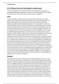
,Lecture 1 + 2 – Intro (Recap) and CH14 (Perfect Market)
All equity project
Suppose a project has 50% to pay 1400 and 50% to pay 900, at costs 800
Expected cash flow = E(CF) = 0.5*1400 + 0.5*900 = 1150
rf is 0.05, Risk premium is 0.10 → rwacc = 0.15
NPV = -I0 + E(CF)/rwacc = -800 + 1150/1.15 = 200 (is 20% of 800)
Using leverage
• If a project is financed partly with debt and partly with equity, we call the equity levered
• The possible returns of levered equity vary more than those of unlevered equity
Levered vs unlevered
• E(Unlevered) = 15% E(Levered)=25%
• Since rf = 0.05, the levered equity requires a double as high risk premium
→ Even though there is still no chance on default!
• WACC does not change under different financing packages
o As debt (which is cheaper than equity) is acquired, cost of equity rises
• No NPV is created by choosing financing package
MM Proposition 1: A (=VU) EU A (=VL) EL
E U = 𝐕 𝐔 = 𝐕 𝐋 = EL + D D
• EU = 𝐕𝐔 since there is no debt, equity equal to the firm value
• 𝐕𝐔 = 𝐕𝐋 no NPV is gained through financing
• 𝐕𝐋 = EL + D the value of the firm is the right side of the balance sheet
• Under perfect capital markets, the unlevered value = the levered value
Leveraged recapitalization
• Using debt to pay dividend to equityholders
• Using debt to buy shares
→ Create debt from equity
→ Recapitalization = changing the capital structure
Example leveraged recapitalization: financing does not affect assets
Assets 200 Equity 200 Cash 80 Debt 80 Cash 0 Debt 80
Assets 200 Equity 200 Assets 200 Equity 120
SV Ondernemingsfinanciering & Vermogensmarkten – Rick Titulaer – 8-6-2022
, 𝑫 𝐸 𝐷
MM2: 𝒓𝑬 = 𝒓𝑼 + (𝒓𝑼 − 𝒓𝑫 ) 𝑬 𝑟 + 𝐸+𝐷 𝑟𝐷 = 𝑟𝑈
𝐸+𝐷 𝐸
rE = market value on levered equity
rU = return on unlevered equity
rD= market value on debt
The cost of levered
MM2 implies there is a linear relation-
ship between rE and the D/E ratio →
Cost of capital budgeting
rU=rA
• Unlevered:
the return of an unlevered company is the return of its assets. (Assets=Liability)
• Levered:
no change in asset free cashflows, so rU is still equal to rA → rE adjusts itself via D/E
Risky debt
Not in all situation, the debtholders (bank) can be repaid with 100%
If the projects is financed by 900 debt, the company cannot repay 945 in the worst scenario.
In that case, the company will default
The bank will require a higher rD → and MM2 still holds
Equity issue and dilution
Dilution: will the profit per share drop when new shares are sold?
Emission → More capital → Projects with positive NPV can be bought
→ Reflected in share price → Current shareholders don’t suffer a loss
SV Ondernemingsfinanciering & Vermogensmarkten – Rick Titulaer – 8-6-2022
, Lecture 3 – CH15 (Debt and taxes)
Disparity
• Debt → Interest → Tax free (tax deductible)
• Equity → Dividend → Tax!
Dutch corporate tax (vpb)
• Debt is tax free
• Double taxation is avoided (deelnemingsvrijstelling)
o Attractive for foreign countries
o Dochter: De winst van de deelneming is onbelast,
Moeder: Winst uit deelneming is onbelast
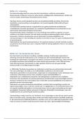
Why use debt, example:
• EBIT = 2500, tax rate = 35%
1) Leverage: 430 interest expenses
430 to debtholders
725 Tax (1776 Total to D+E)
1346 to equityholders
2) No leverage: no interest expenses. 875
0 to debtholders
875 Tax (1625 Total to D+E)
1625 to equity holders
Tax shield
• Arises when there exists debt
• VL=VU+PV(interest tax shield)
The unlevered value is smaller than the levered value (MM1 with tax)
• High debt is advantageous for companies
• The firm effectively borrows at rD(1 - τc) cheaper debt!
Recapitalization
• Is used to get a higher debt to market value rating
• Borrow x as debt, use x from cash to buy own stocks.
𝐷
• R = number of shares repurchased = debt attracted / repurchase price = 𝑷′
• N = number of remaining shares = N0 – R (N0 is the initial # shares)
𝐸𝐿
• P’= 𝑵 , where EL follows from VL = VU + T*D, and EL = VL – D
𝑉 𝑉
• P’ = 𝑁+𝑅
𝐿
= 𝑁𝐿 The equilibrium repurchase price, is the initial value of the firm (levered)
0
• The worth created (NPV) by deducting tax, is given to the shareholder.
Example: rE=0.20 τc=0.35 VU=3.5 mln N0=175.000 → Recap→ rD=0.10, D=1 mln
VL = Vu + PV(interest tax shield) = 3.5 + 0.35*1 = VU + τcD = 3.85
EL = VL – D = 3.85 – 1 = 2.85
P'= 2..000 = 22
R = 1mln / 22 = 45454 shares
SV Ondernemingsfinanciering & Vermogensmarkten – Rick Titulaer – 8-6-2022
𝐸 𝐷
rwacc =𝐸+𝐷 𝑟𝐸 + 𝐸+𝐷 𝑟𝐷 I0 = CapEx + ∆NWC
E(CF) = P(A)*CF(A) + P(B)*CF(B) rp 𝑟𝑓 + (𝐸(𝑅𝑚𝑘𝑡 ) − 𝑟𝑓 )𝛽𝑝
PV = ∑E(CFt) / (1+rwacc)t NPV = PV – I0 = ΔV
𝐸 𝐷
MM1 EU=VU=VL=EL+D MM2 𝑟
𝐸+𝐷 𝐸
+ 𝐸+𝐷 𝑟𝐷 = 𝑟𝑈
MM1 with MM2 with 𝐸 𝐷
tax VL=VU+PV(interest tax shield) tax 𝑟
𝐸+𝐷 𝐸
+ 𝐸+𝐷 𝑟𝐷 (1 − 𝜏𝑐 ) = 𝑟𝑈 = 𝑟𝑤𝑎𝑐𝑐
# Shares
Interest tax 𝐷
shield = (Corporate tax rate) x (Interest payments) repurchas R = debt attracted / rep. price = 𝑃′
ed
Effective tax (1−𝜏𝑐 )(1−𝜏𝑒 ) # Shares
rate 𝜏∗ = 1 − (1−𝜏𝑖 ) remaining N = Ninitial – R
𝑉 𝑉
Cash div cum Pcum = Current div + PV(FCF)
Repurch-
ase price
P’ = 𝑁+𝑅
𝐿
= 𝑁𝐿 (VL=EL+D)
0
Share
Cash div ex Pex = PV(FCF) repurchas Pex = PV(FCF) / (Ninitial – R)
e
Effective tax
(1−𝜏𝑐 )(1−𝜏𝑔 ) Clientele
(Pcum − Pex)(1 − τg) = Div(1 – τd)
retainment 𝜏𝑟∗ = (1 − (1−𝜏𝑖 )
) effect
𝜏𝑑 −𝜏𝑔
Pcum – Pex = Div(1- 1−𝜏 ) = Div(1– τd*)
rate
𝑔
Effective tax (𝜏𝑑 −𝜏𝑔 )
Net Debt = Debt – Cash
dividend rate 𝜏𝑑∗ = Debt
of clientele (1−𝜏𝑔 )
Capacity
𝐷𝑡 = 𝑑 ∗ 𝑉𝑡𝐿
WACC Discount unlevered FCF with rwacc Project
𝐿
𝐹𝐶𝐹𝑡+1 +𝑉𝑡+1
method
(based on net debt) value at t 𝑉𝑡𝐿 = (1+𝑟𝑤𝑎𝑐𝑐 )
Vu=FCF discounted with ru
FTE FCFE = FCF – (1-τc)Interest + 𝛥Debt capacity
APV Method VL=VU + PV(interest tax shield) Method
discounted with ru
Discount PV(FCFE) with re
Profit Call Profit Call
Long max{S-K,0} – C0 Short -max{S-K,0} + C0
Profit Put Profit Put
Long max{K-S,0} – P0 Short -max{K-S,0} + P0
Put-call
parity S+P = C+K Debt parity PV(D) – P
Binomial
Option 𝛥=
𝐶𝑢 −𝐶 𝑑
; 𝐵=
𝐶𝑑 −𝛥𝑆𝑑
; C=𝛥S+B 𝐶 = 𝑆 ∗ 𝑁(𝑑1 ) − 𝑃𝑉(𝐾) ∗ 𝑁(𝑑2 )
Pricing 𝑆𝑢 −𝑆𝑑 1+𝑟𝑓 ln (
𝑆
)
Black- 𝜎√𝑇
𝑃𝑉(𝐾)
Scholes 𝑑1 = 𝜎√𝑇
+ 2
Black- model
Scholes for 𝑃 = −𝑆 ∗ 𝑁(−𝑑1 ) + 𝑃𝑉(𝐾) ∗ 𝑁(−𝑑2 ) (Call) 𝑑2 = 𝑑1 − 𝜎√𝑇
put options
N(…) = cumulative normal density function
Net stock S* = S – PV(Div) = ‘Net’ stock price [or] Replicating 𝛥 = 𝑁(𝑑1 ) and 𝐵 = −𝑃𝑉(𝐾) ∗ 𝑁(𝑑2 ) [put]
price Portfolio
S* = S/(1+q)T with q the dividend yield 𝛥 = −𝑁(−𝑑1 ) and 𝐵 = 𝑃𝑉(𝐾) ∗ 𝑁(−𝑑2 ) [call]
SΔ B 𝑆 Equity 𝐷
Option Beta 𝛽𝐶 = 𝛽 + 𝛽 = Δ𝛽𝑆 Beta 𝛽𝐸 = Δ (1 + ) 𝛽𝑈
𝑆Δ+𝐵 𝑆 𝑆Δ+𝐵 𝐵 𝐶 𝐸
𝐴 𝐸
Unlever-ed 𝛽𝐸 𝛽𝐷 = 𝛽 − 𝐷 𝛽𝐸
𝛽𝑈 = Debt Beta 𝐷 𝑈
Beta
Δ(1 + 𝐷/𝐸)
Cash conver- CCC = Inventory days + Accounts Bench
𝑁𝑃𝑉 1−Δ
sion cycle
mark NPV >
receivable days – Accounts payable days return 𝐼 Δ
Covered 1+𝑟 𝑥
Exchange
interest rate 𝐹 = 𝑆 1+𝑟$ ratio 𝑁𝑇
Parity €
𝑃(𝐿𝑜𝑠𝑠 𝑎𝑡 𝑡)∗𝐸(𝑃𝑎𝑦𝑚𝑒𝑛𝑡 𝑖𝑛 𝑐𝑎𝑠𝑒 𝑜𝑓 𝑙𝑜𝑠𝑠) 𝑃 𝑆
AFIP ∑ Stock swap
NPV>0
Exchange ratio < 𝑃𝑇 (1 + 𝑇)
(1+𝑟𝐿 ) 𝐴
𝑆 𝐾
Garman- 𝐶 = (1+𝑟 )𝑇 ∗ 𝑁(𝑑1 ) − (1+𝑟 )𝑇 ∗ Mortgages Δ𝐷𝐸 ∗𝐸
Kohlhagen 𝐸𝑈𝑅 𝑈𝑆𝐷 to sell
𝐴𝑚𝑜𝑢𝑛𝑡 = Δ𝐷
model 𝐴,𝑓𝑜𝑟 𝑠𝑜𝑙𝑑 𝑎𝑚𝑜𝑢𝑛𝑡
𝑁(𝑑2 )
𝑑𝑃 𝐷 𝑑𝑃 𝐷
Security price = −𝑃 1+𝑟 ; = − 1+𝑟 𝑑𝑟 Duration 𝐴 𝐿
𝑑𝑟 𝑃 𝐷𝐸 = 𝐷𝐴−𝐷 = 𝐷 − 𝐷
sensitivity of Equity 𝐴−𝐿 𝐴 𝐴−𝐿 𝐿
SV Ondernemingsfinanciering & Vermogensmarkten – Rick Titulaer – 8-6-2022
,Lecture 1 + 2 – Intro (Recap) and CH14 (Perfect Market)
All equity project
Suppose a project has 50% to pay 1400 and 50% to pay 900, at costs 800
Expected cash flow = E(CF) = 0.5*1400 + 0.5*900 = 1150
rf is 0.05, Risk premium is 0.10 → rwacc = 0.15
NPV = -I0 + E(CF)/rwacc = -800 + 1150/1.15 = 200 (is 20% of 800)
Using leverage
• If a project is financed partly with debt and partly with equity, we call the equity levered
• The possible returns of levered equity vary more than those of unlevered equity
Levered vs unlevered
• E(Unlevered) = 15% E(Levered)=25%
• Since rf = 0.05, the levered equity requires a double as high risk premium
→ Even though there is still no chance on default!
• WACC does not change under different financing packages
o As debt (which is cheaper than equity) is acquired, cost of equity rises
• No NPV is created by choosing financing package
MM Proposition 1: A (=VU) EU A (=VL) EL
E U = 𝐕 𝐔 = 𝐕 𝐋 = EL + D D
• EU = 𝐕𝐔 since there is no debt, equity equal to the firm value
• 𝐕𝐔 = 𝐕𝐋 no NPV is gained through financing
• 𝐕𝐋 = EL + D the value of the firm is the right side of the balance sheet
• Under perfect capital markets, the unlevered value = the levered value
Leveraged recapitalization
• Using debt to pay dividend to equityholders
• Using debt to buy shares
→ Create debt from equity
→ Recapitalization = changing the capital structure
Example leveraged recapitalization: financing does not affect assets
Assets 200 Equity 200 Cash 80 Debt 80 Cash 0 Debt 80
Assets 200 Equity 200 Assets 200 Equity 120
SV Ondernemingsfinanciering & Vermogensmarkten – Rick Titulaer – 8-6-2022
, 𝑫 𝐸 𝐷
MM2: 𝒓𝑬 = 𝒓𝑼 + (𝒓𝑼 − 𝒓𝑫 ) 𝑬 𝑟 + 𝐸+𝐷 𝑟𝐷 = 𝑟𝑈
𝐸+𝐷 𝐸
rE = market value on levered equity
rU = return on unlevered equity
rD= market value on debt
The cost of levered
MM2 implies there is a linear relation-
ship between rE and the D/E ratio →
Cost of capital budgeting
rU=rA
• Unlevered:
the return of an unlevered company is the return of its assets. (Assets=Liability)
• Levered:
no change in asset free cashflows, so rU is still equal to rA → rE adjusts itself via D/E
Risky debt
Not in all situation, the debtholders (bank) can be repaid with 100%
If the projects is financed by 900 debt, the company cannot repay 945 in the worst scenario.
In that case, the company will default
The bank will require a higher rD → and MM2 still holds
Equity issue and dilution
Dilution: will the profit per share drop when new shares are sold?
Emission → More capital → Projects with positive NPV can be bought
→ Reflected in share price → Current shareholders don’t suffer a loss
SV Ondernemingsfinanciering & Vermogensmarkten – Rick Titulaer – 8-6-2022
, Lecture 3 – CH15 (Debt and taxes)
Disparity
• Debt → Interest → Tax free (tax deductible)
• Equity → Dividend → Tax!
Dutch corporate tax (vpb)
• Debt is tax free
• Double taxation is avoided (deelnemingsvrijstelling)
o Attractive for foreign countries
o Dochter: De winst van de deelneming is onbelast,
Moeder: Winst uit deelneming is onbelast
Why use debt, example:
• EBIT = 2500, tax rate = 35%
1) Leverage: 430 interest expenses
430 to debtholders
725 Tax (1776 Total to D+E)
1346 to equityholders
2) No leverage: no interest expenses. 875
0 to debtholders
875 Tax (1625 Total to D+E)
1625 to equity holders
Tax shield
• Arises when there exists debt
• VL=VU+PV(interest tax shield)
The unlevered value is smaller than the levered value (MM1 with tax)
• High debt is advantageous for companies
• The firm effectively borrows at rD(1 - τc) cheaper debt!
Recapitalization
• Is used to get a higher debt to market value rating
• Borrow x as debt, use x from cash to buy own stocks.
𝐷
• R = number of shares repurchased = debt attracted / repurchase price = 𝑷′
• N = number of remaining shares = N0 – R (N0 is the initial # shares)
𝐸𝐿
• P’= 𝑵 , where EL follows from VL = VU + T*D, and EL = VL – D
𝑉 𝑉
• P’ = 𝑁+𝑅
𝐿
= 𝑁𝐿 The equilibrium repurchase price, is the initial value of the firm (levered)
0
• The worth created (NPV) by deducting tax, is given to the shareholder.
Example: rE=0.20 τc=0.35 VU=3.5 mln N0=175.000 → Recap→ rD=0.10, D=1 mln
VL = Vu + PV(interest tax shield) = 3.5 + 0.35*1 = VU + τcD = 3.85
EL = VL – D = 3.85 – 1 = 2.85
P'= 2..000 = 22
R = 1mln / 22 = 45454 shares
SV Ondernemingsfinanciering & Vermogensmarkten – Rick Titulaer – 8-6-2022