3.3. Predicting the outcome of a variable
Exploring the relationship between 2 quantitative variables graphically scatterplot
Straight-line pattern? correlation coefficient describes its strength numerically
Further analysis finding an equation for the straight line that best describes that pattern
This equation can be used to predict the value of the variable designated as the response variable
from the value of the variable designated as the explanatory variable.
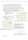
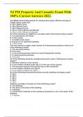
Regression line = predicts the value for the response variable y as a straight-line function of the
value x of the explanatory variable. Let ^y denote the predicted value of y.
- The equation for the regression line has
the form: ^y =a+bx
- a denotes the y-intercept and b denotes
the slope.
y-intercept = the predicted value of y when x = 0
slope = equals the amount that ^y changes when
x increases by one unit.
- For two x values that differ by 1.0, the ^y
values differ by b.
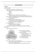
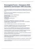
When the slope is negative ^y decreases as x
increases. The straight line then goes downward,
and the association is negative.
When the slope = 0, the regression line is
horizontal (parallel to the x-axis). ^y stays constant
at the y-intercept for any value of x. ^y does not
change as x changes and the variables don’t
exhibit association.
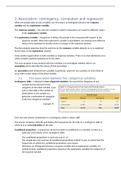
, The absolute value of the slope describes the magnitude of the change in ^y for a 1-unit change in x.
The larger the absolute value, the steeper the regression line.
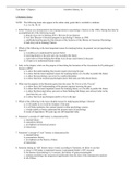
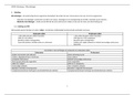
Prediction error / residuals = difference between the actual y value and the predicted y value.
Residual = y− ^y
Each observation has a residual
A positive residual occurs when the actual y is larger than ^y , so that y− ^y > 0
A negative residual results when the actual y is smaller than ^y , so that y− ^y < 0
The smaller the absolute value of the residual, the closer the predicted value is to the actual value,
so the better the prediction.
If the predicted value is the same as the actual value, the residual is zero: y− ^y =0
In a scatterplot, the vertical distance between the point and the regression line is the absolute value
of the residual.
How is the equation for the regression line found?
The actual summary measure used to evaluate regression lines is called the residual sum of squares
residual ∑ of squares=Σ( residual)2=Σ( y− ^y )2
This formula squares each vertical distance between a point and the line and then adds up these
squared values. The better the line, the smaller the residuals tend to be, and the smaller the residual
sum of squares tends to be.
For each potential line, we have a set of predicted values, a set of residuals and a residual sum of
squares. The line that the software reports is the one having the smallest residual sum of squares.
This is why selecting a line is called the least squares method.
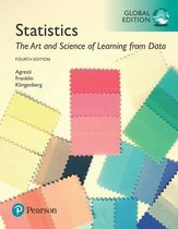
This regression line:
- Makes the errors as small as possible
- Has some positive residuals and some negative residuals, and the sum (and mean) of the
residuals equals 0
o Too-high predictions are balanced by too-low predictions
- Passes through the point ( x , y )
o The center of the data
sy
Formula for slope is b=r ( )
sx
Formula for y-intercept is a= y−b( x)
The slope b is directly related to the correlation r and the y-intercept depends on the slope.
We’ve used correlation to describe the strength of the association.
Exploring the relationship between 2 quantitative variables graphically scatterplot
Straight-line pattern? correlation coefficient describes its strength numerically
Further analysis finding an equation for the straight line that best describes that pattern
This equation can be used to predict the value of the variable designated as the response variable
from the value of the variable designated as the explanatory variable.
Regression line = predicts the value for the response variable y as a straight-line function of the
value x of the explanatory variable. Let ^y denote the predicted value of y.
- The equation for the regression line has
the form: ^y =a+bx
- a denotes the y-intercept and b denotes
the slope.
y-intercept = the predicted value of y when x = 0
slope = equals the amount that ^y changes when
x increases by one unit.
- For two x values that differ by 1.0, the ^y
values differ by b.
When the slope is negative ^y decreases as x
increases. The straight line then goes downward,
and the association is negative.
When the slope = 0, the regression line is
horizontal (parallel to the x-axis). ^y stays constant
at the y-intercept for any value of x. ^y does not
change as x changes and the variables don’t
exhibit association.
, The absolute value of the slope describes the magnitude of the change in ^y for a 1-unit change in x.
The larger the absolute value, the steeper the regression line.
Prediction error / residuals = difference between the actual y value and the predicted y value.
Residual = y− ^y
Each observation has a residual
A positive residual occurs when the actual y is larger than ^y , so that y− ^y > 0
A negative residual results when the actual y is smaller than ^y , so that y− ^y < 0
The smaller the absolute value of the residual, the closer the predicted value is to the actual value,
so the better the prediction.
If the predicted value is the same as the actual value, the residual is zero: y− ^y =0
In a scatterplot, the vertical distance between the point and the regression line is the absolute value
of the residual.
How is the equation for the regression line found?
The actual summary measure used to evaluate regression lines is called the residual sum of squares
residual ∑ of squares=Σ( residual)2=Σ( y− ^y )2
This formula squares each vertical distance between a point and the line and then adds up these
squared values. The better the line, the smaller the residuals tend to be, and the smaller the residual
sum of squares tends to be.
For each potential line, we have a set of predicted values, a set of residuals and a residual sum of
squares. The line that the software reports is the one having the smallest residual sum of squares.
This is why selecting a line is called the least squares method.
This regression line:
- Makes the errors as small as possible
- Has some positive residuals and some negative residuals, and the sum (and mean) of the
residuals equals 0
o Too-high predictions are balanced by too-low predictions
- Passes through the point ( x , y )
o The center of the data
sy
Formula for slope is b=r ( )
sx
Formula for y-intercept is a= y−b( x)
The slope b is directly related to the correlation r and the y-intercept depends on the slope.
We’ve used correlation to describe the strength of the association.