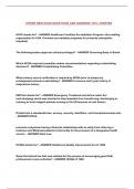
CONSUMPTION AND SAVING SCHEDULE
CHAPTER 13 • 45o line: line along which the value of GDP is
basic macroeconomic relationships equal to the value of aggregate expenditures
• a – consumption rises as income increases
ASSUMPTIONS AND SIMPLIFICATIONS o saving is negative when consumption
1. Stuck-Price Model schedule is above 45o line
o saving is positive when consumption
• assumption that prices are fixed
schedule is below 45o line
2. Unplanned Inventory Changes
o at each point on the 45o line,
• inventories either rise/fall more than consumption = disposable income
intended because demand is either • b – saving increases as income goes up
unexpectedly high/low o saving schedule is found by
• the one that allows it to achieve equilibrium - subtracting consumption schedule in
production decisions are made in response to vertically from 45o lie
unexpected changes in inventory levels • saving is zero where consumption equals
• inventory rising – cut back on productions disposable income
• inventory falling – increase production • dissaving:
3. Introduction and relevance o vertical distance of consumption
• model remains relevant today – many prices schedule above 45o line
are inflexible downward over relatively short o vertical distance of saving schedule
periods of time below horizontal axis
• model helps us understand how modern • break-even income: level of disposable
economy is likely to adjust to various income at which households plan to consume
economic shocks over shorter periods of time all their income ( C = Yd)
INCOME-CONSUMPTIONS AND INCOME-SAVING
• income-consumption: the more the
consumers earn, the more they spend
• income-savings: the more the consumers
earn, the more income they can save
• savings: not spending or the part of
disposable income not consumed
o Yd = C + S
o S = Yd – C
o C = Yd – S
• main factor to determine nation’s levels of
consumptions and saving – disposable MARGINAL PROPENSITIES
income • marginal propensity to consume: portion of
change in income that is consumed
CONSUMPTION AND SAVING SCHEDULES !"#$%& ($ !)$*+,-.()$
o MPC = !"#$%& ($ ($!),&
• consumption schedule: shows amounts
• marginal propensity to save: portion of
households plan to spend on consumer goods
change in income that is saved
at different levels of disposable income !"#$%& ($ *#/($%
• saving schedule: shows amounts households o MPS = !"#$%& ($ ($!),&
plan to save at different levels of disposable • MPC + MPS = 1
income o MPC = 1 – MPS
o MPS = 1 -MPC
1
, MPC AND MPS AS SLOPES o real interest rates:
• MPC: numerical value of the slope of the § interest rate falls: households
consumption schedule borrow more, consume more
• MPS: numerical value of the slope of the and save less
saving schedule o household debt: household debt as %
of disposable income is held constant
§ increased borrowing shifts
consumption schedule up
§ reduced borrowings shift
consumption schedule down
THE INTEREST RATE-INVESTMENT RELATIONSHIP
1. Expected Rate of Return (r)
• the increase in profit firm anticipates it will
obtain by purchasing capital, expressed as %
of the total cost of the investment activity
• MPC is slope of consumption schedule • not guaranteed rate of return
• MPS is slope of saving schedule 2. The Real Interest Rate (i)
• nominal interest rate – inflation rate
EXOGENEOUS CONSUMPTION AND SAVING • matters for investment decisions
• the aggregate amount of money spent by • r > i – investment should be undertaken
consumers when income is zero • r < i – investment should not be undertaken
o Y = 0 then C = C0, S = -C0 • r = i – firms undertake investment decisions
• variables that determine schedules: up until this point and not where r is below i
o disposable income 3. Investment Demand Curve
§ C = Yd • curve that shows amounts of investment
§ S = Yd - C demanded by economy at series of real
o MPC and MPS interest rates
§ C = cYd • constructed by arraying all potential
§ S = (1-c)Yd investment projects in descending order of
o exogenous consumption C0 their expected rates of return
§ C = C0 + cYd • curve slopes downward – reflects inverse
§ S = -C0 + (1-c)Yd relationship between real interest rate and
• non-income determinants: quantity of investment demanded
o wealth: value of real and financial • curve ID is economy’s investment demand
assets that household owns curve
§ wealth effect: tendency for • increase in investment: curve shifts to right
people to increase their • decrease in investment: curve shifts to left
consumption spending when
value of their financial and
real assets rises, and to
decrease their consumption
spending when value of those
assets falls
o expectations: household expectations
about future prices and income may
affect current spending and saving
2