Research Methods in Finance Lectures – University of Groningen – Joris Wellen
Research Methods in Finance
Lectures
Summary of the course’s lectures
Joris Wellen – University of Groningen
Content
Lecture 1 – A Quick Look at OLS..................................................................................................................... 3
1.1 Course Information.........................................................................................................................................3
1.2 Ordinary Least Squares (OLS).........................................................................................................................3
Lecture 2 – OLS Assumptions and Diagnostic Tests.......................................................................................11
2.1 Gauss-Markov Assumptions.........................................................................................................................11
2.2 Detecting Autocorrelation: the Durbin-Watson test....................................................................................13
2.3 Five Cases in which Assumption 4 is Not Satisfied.......................................................................................15
Lecture 3 – Dummies to the Right, Dummies to the Left...............................................................................16
3.1 Dummy Variables.........................................................................................................................................16
3.2 Dummies on the Right..................................................................................................................................16
3.3 Dummies on the Left....................................................................................................................................20
Lecture 4 – Time Series................................................................................................................................ 26
4.1 Introduction..................................................................................................................................................26
4.2 Univariate Time Series..................................................................................................................................26
4.3 Stationarity...................................................................................................................................................27
4.4 Autoregressive Models.................................................................................................................................29
4.5 Testing for Non-Stationarity.........................................................................................................................31
4.6 Financial Bubbles..........................................................................................................................................36
Lecture 5 – Modelling Volatility: ARCH, GARCH and E-GARCH.......................................................................37
5.1 Introduction..................................................................................................................................................37
5.2 Autoregressive Conditional Heteroscedasticity (ARCH) Models..................................................................38
5.3 Generalized ARCH (GARCH) Models.............................................................................................................40
5.4 The E-GARCH Model.....................................................................................................................................44
Lecture 6 – Panel Data................................................................................................................................. 45
6.1 Introduction..................................................................................................................................................45
6.2 Panel Data....................................................................................................................................................45
6.3 Fixed Effects and Random Effects................................................................................................................46
6.4 Random effects.............................................................................................................................................51
1
, Research Methods in Finance Lectures – University of Groningen – Joris Wellen
Lecture 7 – Course Recap............................................................................................................................. 54
7.1 Panel-level Heteroscedasticity.....................................................................................................................54
7.2 Panel-level autocorrelation..........................................................................................................................54
7.3 Clustered Standard Errors............................................................................................................................54
7.4 The Course....................................................................................................................................................55
2
, Research Methods in Finance Lectures – University of Groningen – Joris Wellen
Lecture 1 – A Quick Look at OLS
1.1 Course Information
Exam consists of 3rd of lecture 4.
Steffen prefers short and to-the-point answers
Steffen prefers good tables
1.2 Ordinary Least Squares (OLS)
OLS and stuff
1. A quick overview of the OLS estimator
2. How do we estimate unkown parameters in the regression model?
Ordinary leas squares (OLS).
3. What are the properties of the OLS estimator?
4. No properties without assumptions.
5. When all assumptions are correct, OLS is the best estimator we can
use.
Following supplementary material is available on Nestor and (link)
Hypothesis testing in linear regression models, R2 and more.
Regression is concerned with describing and evaluating the relationship
between a given variable and one or more other variables.
Examples:
1. How do asset returns vary with their level of market risk?
2. What factors impact the price or demand for a good?
Regression <<>> correlation
Correlation: measures the degree of linear association between two
variables They are treated systematically.
Regression: The dependent variable, Y, is treated differently than the
independent variable(s), x. y is assumed to be random/stochastic,
whereas x is assumed to be fixed/non-stochastic.
An example a simple regression
Suppose we want to study the relationship between the excess returns on
a fund manager’s portfolio (‘fund XXX’) and the excess return on a market
index.
3
, Research Methods in Finance Lectures – University of Groningen – Joris Wellen
A simple linear regression can easily be extended to include k-1
explanatory variables
In general, we have three types of data:
1. Cross-sectional data
y i=α + β x i + ε i
2. Time-series data
y t =α + β x t + ε t
3. Panel data
y ¿ =α+ β x ¿ + ε ¿
The random error component U t can capture a number of features.
1. We always leave out some determinants of Y t (example: IQ)
2. There may be error in the measurement of Y t that cannot be
modelled
3. Random outside influences on Y t which we cannot model (a terrorist
attack, a natural disaster, a double rainbow.
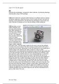
How did we estimate the line from the picture below?
Y t =α + β x t +u
- The most common method used to fit a line, and estimate α and β is
Ordinary Least Squares (OLS).
- OLS tries to minimize the sum of squared residuals.
Ordinary Least
Squares (OLS):
4
Research Methods in Finance
Lectures
Summary of the course’s lectures
Joris Wellen – University of Groningen
Content
Lecture 1 – A Quick Look at OLS..................................................................................................................... 3
1.1 Course Information.........................................................................................................................................3
1.2 Ordinary Least Squares (OLS).........................................................................................................................3
Lecture 2 – OLS Assumptions and Diagnostic Tests.......................................................................................11
2.1 Gauss-Markov Assumptions.........................................................................................................................11
2.2 Detecting Autocorrelation: the Durbin-Watson test....................................................................................13
2.3 Five Cases in which Assumption 4 is Not Satisfied.......................................................................................15
Lecture 3 – Dummies to the Right, Dummies to the Left...............................................................................16
3.1 Dummy Variables.........................................................................................................................................16
3.2 Dummies on the Right..................................................................................................................................16
3.3 Dummies on the Left....................................................................................................................................20
Lecture 4 – Time Series................................................................................................................................ 26
4.1 Introduction..................................................................................................................................................26
4.2 Univariate Time Series..................................................................................................................................26
4.3 Stationarity...................................................................................................................................................27
4.4 Autoregressive Models.................................................................................................................................29
4.5 Testing for Non-Stationarity.........................................................................................................................31
4.6 Financial Bubbles..........................................................................................................................................36
Lecture 5 – Modelling Volatility: ARCH, GARCH and E-GARCH.......................................................................37
5.1 Introduction..................................................................................................................................................37
5.2 Autoregressive Conditional Heteroscedasticity (ARCH) Models..................................................................38
5.3 Generalized ARCH (GARCH) Models.............................................................................................................40
5.4 The E-GARCH Model.....................................................................................................................................44
Lecture 6 – Panel Data................................................................................................................................. 45
6.1 Introduction..................................................................................................................................................45
6.2 Panel Data....................................................................................................................................................45
6.3 Fixed Effects and Random Effects................................................................................................................46
6.4 Random effects.............................................................................................................................................51
1
, Research Methods in Finance Lectures – University of Groningen – Joris Wellen
Lecture 7 – Course Recap............................................................................................................................. 54
7.1 Panel-level Heteroscedasticity.....................................................................................................................54
7.2 Panel-level autocorrelation..........................................................................................................................54
7.3 Clustered Standard Errors............................................................................................................................54
7.4 The Course....................................................................................................................................................55
2
, Research Methods in Finance Lectures – University of Groningen – Joris Wellen
Lecture 1 – A Quick Look at OLS
1.1 Course Information
Exam consists of 3rd of lecture 4.
Steffen prefers short and to-the-point answers
Steffen prefers good tables
1.2 Ordinary Least Squares (OLS)
OLS and stuff
1. A quick overview of the OLS estimator
2. How do we estimate unkown parameters in the regression model?
Ordinary leas squares (OLS).
3. What are the properties of the OLS estimator?
4. No properties without assumptions.
5. When all assumptions are correct, OLS is the best estimator we can
use.
Following supplementary material is available on Nestor and (link)
Hypothesis testing in linear regression models, R2 and more.
Regression is concerned with describing and evaluating the relationship
between a given variable and one or more other variables.
Examples:
1. How do asset returns vary with their level of market risk?
2. What factors impact the price or demand for a good?
Regression <<>> correlation
Correlation: measures the degree of linear association between two
variables They are treated systematically.
Regression: The dependent variable, Y, is treated differently than the
independent variable(s), x. y is assumed to be random/stochastic,
whereas x is assumed to be fixed/non-stochastic.
An example a simple regression
Suppose we want to study the relationship between the excess returns on
a fund manager’s portfolio (‘fund XXX’) and the excess return on a market
index.
3
, Research Methods in Finance Lectures – University of Groningen – Joris Wellen
A simple linear regression can easily be extended to include k-1
explanatory variables
In general, we have three types of data:
1. Cross-sectional data
y i=α + β x i + ε i
2. Time-series data
y t =α + β x t + ε t
3. Panel data
y ¿ =α+ β x ¿ + ε ¿
The random error component U t can capture a number of features.
1. We always leave out some determinants of Y t (example: IQ)
2. There may be error in the measurement of Y t that cannot be
modelled
3. Random outside influences on Y t which we cannot model (a terrorist
attack, a natural disaster, a double rainbow.
How did we estimate the line from the picture below?
Y t =α + β x t +u
- The most common method used to fit a line, and estimate α and β is
Ordinary Least Squares (OLS).
- OLS tries to minimize the sum of squared residuals.
Ordinary Least
Squares (OLS):
4