1. Comment
7 December 2019 at 13:48:58
Median of lower half
2. Comment
7 December 2019 at 13:49:07
Medium of upper half
Statistics 1: Description and
Inference
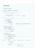
Lecture 1 - Distributions, Means and Deviations
Variable: anything that can be measured and can differ across entities across time
• Independent (x): cause, doesn’t change
• Dependent (y): outcome, does changes
Levels of measurement:
• Categorical
• Nominal: no natural order
• Ordinal: natural order/rank
• Continuous vs discrete:
• Interval: 0 is arbitrary (e.g. °C)
• Ratio: 0 is meaningful (e.g. Kelvin)
Frequency distributions:
• Measure of central tendency: central position of data set
• Mean: average of numbers
n
∑i=1 xi
• x̄ =
n
• μ: mean of population
• x̄: mean of sample
• Sensitive to extreme values/outliers
• Median: middle score when data is arranged by magnitude
• Mode: most frequent score
• Measure of dispersion: stretch/squeeze of data set
• Range: maximum value - minimum value
• Interquartile range (IQR): range of middle 50%
1 2 • Q3 - Q1
• Deviance: how much does data deviate from mean
n
SS ∑ (xi − x̄ )2
2
• Variance: s = = i=1
N−1 N−1
• SS: sum of squared errors
• Standard deviation: s = var i a n ce
• σ: standard deviation of population
• s: standard deviation of sample
• Normal distribution: where mean = median = mode (symmetrical), allow us to calculate
probabilities of outcome values
• Ranges:
• 68% within 1σ of μ
• 95% within 1.96σ of μ
,3. Comment
7 December 2019 at 15:10:34
Multiple of σ (e.g. 1.96)
4. Comment
7 December 2019 at 14:08:27
Don’t do both smaller or both
larger
5. Comment
9 December 2019 at 12:40:50
When categories are not
substituted by numbers
6. Comment
7 December 2019 at 14:22:47 • 99.7% within 3σ of μ
Instead of computed as 0. • Standardizing normal distribution:
x − x̄
3 • Z-score: z =
Missing values given random s
number (e.g. -8) in data view, • Refer to table of standard normal distribution to identify probability
which is identified as value to be • Finding ranges:
excluded in variable view. • If both values on same side of mean, subtract like normal
4 • If each value on either side, choose one larger and one smaller portion and subtract
7. Comment
7 December 2019 at 14:30:16
Opens up syntax
SPSS 1
Necessary to prevent technical
issues? Windows:
• Data editor: input data
8. Comment • Tabs:
7 December 2019 at 14:30:32
• Variable View: defining variables (and their characteristics)
Opens up output/viewer 5 • Type: numeric, string (categorical)
• Label: full name of variable
• Values: allows categories to be represented as numbers
6 • Missing: identifies values to be excluded from data
• Measure: scale (interval-ratio), ordinal, nominal
• Data View: defining values within each variable
• Output/viewer: interpret data (displays graphs, tables, special values)
Analyzing frequency distributions:
[Analyze] → [Descriptive Statistics] → [Frequencies] → select variable(s) → click arrow →
7 8 [Statistics…] → choose measures → [Continue] → [Paste] → click play
, 9. Comment
7 December 2019 at 14:38:07
Expected
10. Comment
7 December 2019 at 14:38:13
Observed
11. Comment
7 December 2019 at 14:38:50
E.g. deviance
12. Comment
7 December 2019 at 14:34:43
Measured data
13. Comment Lecture 2 ??
7 December 2019 at 14:34:55
Estimated data (from variables) Statistical models: summarize data (observed) and predict real world (expected)
14. Comment 9 11 outcomei = (model) + errori
7 December 2019 at 15:01:51
12 13 • Combination of variables and parameters
Where means of samples are
there own data values
Goodness of fit:
• Tradeoff between simplicity and accuracy
15. Comment n
SS ∑ (outcom ei − m od eli )2
7 December 2019 at 15:07:55
• m ea n squ ared er r or (MSE ) = = i=1
Most normal. N−1 d egrees of f reed om
• Aka variance (more general)
Interval range in which 95% of • Degrees of freedom = N - 1
sample means fall. • outcomei = xi
• modeli = x̄
Or there Is 5% chance that range • outcomei = b0 + b1xi + errori
does not include population • Quadratic equation (y = ax + b + errori)
mean
Sampling:
16. Comment • Samples: estimated population parameters
7 December 2019 at 15:09:52 • Allow us to generalize about population
From Z-score. • Sampling distribution: theoretical distribution of infinite samples
• Central limit theorem: when samples become large, average of sample means = population
17. Comment mean
7 December 2019 at 15:19:34 • Approximately normally distributed
More prone to produce values far 14 • Standard error (σx̄ ): standard deviation of sampling distribution
from mean s
σx̄ =
• N
18. Comment • Con dence interval: range in which true population mean likely exists
7 December 2019 at 15:20:40 • Format: CI = {lower bound; upper bound}
As N increases, t-distribution • CI = x̄ ± threshold value × σx̄
more similar to normal 15 • Usually 90%, 95%, 99%
distribution. • Higher CIs are wider ranges
• Using z-score (sample > 100):
16 • 95% CI = x̄ ± 1.96 × σx̄
• Central limit theorem allows us to use z-score
• Using t-distribution (sample < 100)
17 • Symmetric/bell-shaped (like normal distribution) but heavier tails
18 • Shape depends on degrees of freedom (df = N - 1)
• CI = x̄ ± tN-1 × σx̄
• tN-1 found in table of t-distribution
SPSS 2
fi
7 December 2019 at 13:48:58
Median of lower half
2. Comment
7 December 2019 at 13:49:07
Medium of upper half
Statistics 1: Description and
Inference
Lecture 1 - Distributions, Means and Deviations
Variable: anything that can be measured and can differ across entities across time
• Independent (x): cause, doesn’t change
• Dependent (y): outcome, does changes
Levels of measurement:
• Categorical
• Nominal: no natural order
• Ordinal: natural order/rank
• Continuous vs discrete:
• Interval: 0 is arbitrary (e.g. °C)
• Ratio: 0 is meaningful (e.g. Kelvin)
Frequency distributions:
• Measure of central tendency: central position of data set
• Mean: average of numbers
n
∑i=1 xi
• x̄ =
n
• μ: mean of population
• x̄: mean of sample
• Sensitive to extreme values/outliers
• Median: middle score when data is arranged by magnitude
• Mode: most frequent score
• Measure of dispersion: stretch/squeeze of data set
• Range: maximum value - minimum value
• Interquartile range (IQR): range of middle 50%
1 2 • Q3 - Q1
• Deviance: how much does data deviate from mean
n
SS ∑ (xi − x̄ )2
2
• Variance: s = = i=1
N−1 N−1
• SS: sum of squared errors
• Standard deviation: s = var i a n ce
• σ: standard deviation of population
• s: standard deviation of sample
• Normal distribution: where mean = median = mode (symmetrical), allow us to calculate
probabilities of outcome values
• Ranges:
• 68% within 1σ of μ
• 95% within 1.96σ of μ
,3. Comment
7 December 2019 at 15:10:34
Multiple of σ (e.g. 1.96)
4. Comment
7 December 2019 at 14:08:27
Don’t do both smaller or both
larger
5. Comment
9 December 2019 at 12:40:50
When categories are not
substituted by numbers
6. Comment
7 December 2019 at 14:22:47 • 99.7% within 3σ of μ
Instead of computed as 0. • Standardizing normal distribution:
x − x̄
3 • Z-score: z =
Missing values given random s
number (e.g. -8) in data view, • Refer to table of standard normal distribution to identify probability
which is identified as value to be • Finding ranges:
excluded in variable view. • If both values on same side of mean, subtract like normal
4 • If each value on either side, choose one larger and one smaller portion and subtract
7. Comment
7 December 2019 at 14:30:16
Opens up syntax
SPSS 1
Necessary to prevent technical
issues? Windows:
• Data editor: input data
8. Comment • Tabs:
7 December 2019 at 14:30:32
• Variable View: defining variables (and their characteristics)
Opens up output/viewer 5 • Type: numeric, string (categorical)
• Label: full name of variable
• Values: allows categories to be represented as numbers
6 • Missing: identifies values to be excluded from data
• Measure: scale (interval-ratio), ordinal, nominal
• Data View: defining values within each variable
• Output/viewer: interpret data (displays graphs, tables, special values)
Analyzing frequency distributions:
[Analyze] → [Descriptive Statistics] → [Frequencies] → select variable(s) → click arrow →
7 8 [Statistics…] → choose measures → [Continue] → [Paste] → click play
, 9. Comment
7 December 2019 at 14:38:07
Expected
10. Comment
7 December 2019 at 14:38:13
Observed
11. Comment
7 December 2019 at 14:38:50
E.g. deviance
12. Comment
7 December 2019 at 14:34:43
Measured data
13. Comment Lecture 2 ??
7 December 2019 at 14:34:55
Estimated data (from variables) Statistical models: summarize data (observed) and predict real world (expected)
14. Comment 9 11 outcomei = (model) + errori
7 December 2019 at 15:01:51
12 13 • Combination of variables and parameters
Where means of samples are
there own data values
Goodness of fit:
• Tradeoff between simplicity and accuracy
15. Comment n
SS ∑ (outcom ei − m od eli )2
7 December 2019 at 15:07:55
• m ea n squ ared er r or (MSE ) = = i=1
Most normal. N−1 d egrees of f reed om
• Aka variance (more general)
Interval range in which 95% of • Degrees of freedom = N - 1
sample means fall. • outcomei = xi
• modeli = x̄
Or there Is 5% chance that range • outcomei = b0 + b1xi + errori
does not include population • Quadratic equation (y = ax + b + errori)
mean
Sampling:
16. Comment • Samples: estimated population parameters
7 December 2019 at 15:09:52 • Allow us to generalize about population
From Z-score. • Sampling distribution: theoretical distribution of infinite samples
• Central limit theorem: when samples become large, average of sample means = population
17. Comment mean
7 December 2019 at 15:19:34 • Approximately normally distributed
More prone to produce values far 14 • Standard error (σx̄ ): standard deviation of sampling distribution
from mean s
σx̄ =
• N
18. Comment • Con dence interval: range in which true population mean likely exists
7 December 2019 at 15:20:40 • Format: CI = {lower bound; upper bound}
As N increases, t-distribution • CI = x̄ ± threshold value × σx̄
more similar to normal 15 • Usually 90%, 95%, 99%
distribution. • Higher CIs are wider ranges
• Using z-score (sample > 100):
16 • 95% CI = x̄ ± 1.96 × σx̄
• Central limit theorem allows us to use z-score
• Using t-distribution (sample < 100)
17 • Symmetric/bell-shaped (like normal distribution) but heavier tails
18 • Shape depends on degrees of freedom (df = N - 1)
• CI = x̄ ± tN-1 × σx̄
• tN-1 found in table of t-distribution
SPSS 2
fi