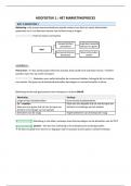
Measurem Step 1: Defining the
Explanation Step 2: Designing the model Step 3: Checking Assumptions
ent: objectives
Test whether non metric IV's
lead to different levels for a 1. Are the observations independent? The
set of metric outcome treatment variable should only refer to 1 level
variables. The dependent 1.Sample size: at least 20 of treatment variable. If not > use repeated
variable is metric. - observations per cell. measures ANOVA.
2. Are all variances equal across treatment
1 way ANOVA = more than 2 2.Treatments and interactions: variables?
population, 1 factor(IV), 1 decide how many variables - check for homoscedasticity using Levene's
Test whether non
DV. and interactions. Test. If this assumption is rejected > I. if the
metric IV's lead to
sample size is equall accross all treatment
different levels for a set
- N way ANOVA = more than 3. Use of covariates: problems, there is no problem if not >
Anova of metric outcome
2 population, more than 1 covariates act like control Transform the DV into logarithm and test
variables. The
factor, 1 DV. variables and help to identify again, if still not > adjust the cut off for
dependent variable is
and measure the effect of the significance.
metric.
- MANOVA = more than 2 treatment variables. 3. Is the dependent variable normally
population, more than 1 Covariates should be: distrubuted?
factor, more than 1 DV. continous, pre-measured, - Check for normality using Kolmogrov Smirnov
independent of treatment, or Shapiro-Wilk test. If not > if the sample is
ANOVA overcomes the limited number. large, this is not a problem. If not > transform
multiple testing problem the DV to make the distribution more
which is the chances of a symmetric. Sample size cutoff point is 30.
type 1 error.
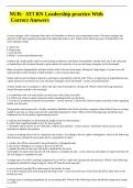
, Step 4: Estimation the model OR Derive Step 6: Validating
Step 5: Interpretating the results
the factors/clusters the results
1. Impact of interaction: when 2 variables are combined.
Does the impact of a change in one trearment variable
depend on the level of the other treatment variable. Type
of interaction:
- Ordinal: the magnitude of one IV depends on the other,
but direction also depends on the other IV.
- Disordinal: Also the direction depends on the other IV.
Estimating the model
2. Significance of main effects:
Anova calculations:
- disordinal interaction, it does not make sense to check
Xg = group average.
main effects.
X = overall average. Consider
- no interaction or ordinal, it is.
SSBg = sum squared between groups = validation tests
3. Impact of covariates > not interesting.
ng(Xg-X)^2 through control
4. Effect size: partial ETA squared = % of variance
MMSB = mean SSB =. 1/G-1 *G*SSBg variables
explained by IV. R2 check the full variance while ETA
MSSW=mean sum of squares within group. Replicate study
checks per variable.
F value = MSSB/MSSW. Asses whether
5. Direction and signifcance of specific population
variation between group is larger than the
differences.
variation within groups.
- Checking for the mean, if mean is higher means there is
higher effect. 2 approaches to check where the effect
comes from:
- Planned comparison: compare the differences and check
the P value. Several tests needed.
-Post hoc: compares everything to everything. Prevents
multiple testing problem.
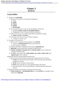
Explanation Step 2: Designing the model Step 3: Checking Assumptions
ent: objectives
Test whether non metric IV's
lead to different levels for a 1. Are the observations independent? The
set of metric outcome treatment variable should only refer to 1 level
variables. The dependent 1.Sample size: at least 20 of treatment variable. If not > use repeated
variable is metric. - observations per cell. measures ANOVA.
2. Are all variances equal across treatment
1 way ANOVA = more than 2 2.Treatments and interactions: variables?
population, 1 factor(IV), 1 decide how many variables - check for homoscedasticity using Levene's
Test whether non
DV. and interactions. Test. If this assumption is rejected > I. if the
metric IV's lead to
sample size is equall accross all treatment
different levels for a set
- N way ANOVA = more than 3. Use of covariates: problems, there is no problem if not >
Anova of metric outcome
2 population, more than 1 covariates act like control Transform the DV into logarithm and test
variables. The
factor, 1 DV. variables and help to identify again, if still not > adjust the cut off for
dependent variable is
and measure the effect of the significance.
metric.
- MANOVA = more than 2 treatment variables. 3. Is the dependent variable normally
population, more than 1 Covariates should be: distrubuted?
factor, more than 1 DV. continous, pre-measured, - Check for normality using Kolmogrov Smirnov
independent of treatment, or Shapiro-Wilk test. If not > if the sample is
ANOVA overcomes the limited number. large, this is not a problem. If not > transform
multiple testing problem the DV to make the distribution more
which is the chances of a symmetric. Sample size cutoff point is 30.
type 1 error.
, Step 4: Estimation the model OR Derive Step 6: Validating
Step 5: Interpretating the results
the factors/clusters the results
1. Impact of interaction: when 2 variables are combined.
Does the impact of a change in one trearment variable
depend on the level of the other treatment variable. Type
of interaction:
- Ordinal: the magnitude of one IV depends on the other,
but direction also depends on the other IV.
- Disordinal: Also the direction depends on the other IV.
Estimating the model
2. Significance of main effects:
Anova calculations:
- disordinal interaction, it does not make sense to check
Xg = group average.
main effects.
X = overall average. Consider
- no interaction or ordinal, it is.
SSBg = sum squared between groups = validation tests
3. Impact of covariates > not interesting.
ng(Xg-X)^2 through control
4. Effect size: partial ETA squared = % of variance
MMSB = mean SSB =. 1/G-1 *G*SSBg variables
explained by IV. R2 check the full variance while ETA
MSSW=mean sum of squares within group. Replicate study
checks per variable.
F value = MSSB/MSSW. Asses whether
5. Direction and signifcance of specific population
variation between group is larger than the
differences.
variation within groups.
- Checking for the mean, if mean is higher means there is
higher effect. 2 approaches to check where the effect
comes from:
- Planned comparison: compare the differences and check
the P value. Several tests needed.
-Post hoc: compares everything to everything. Prevents
multiple testing problem.