Finite Element Method
The basic idea in the finite element method is to find the solution of a complicated
problem by replacing it with a simpler one. Since the actual problem is replaced by
a simpler one in finding the solution, we will be able to find only an approximate
solution rather than the exact solution. The existing mathematical tools will not be
sufficient to find the exact solution (and sometimes, even an approximate solution)
of most of the practical problems. Thus, in the absence of any other convenient
method to find even the approximate solution of a given problem, we have to prefer
the finite element method. Moreover, in the finite element method, it will often be
possible to improve or refine the approximate solution by spending more
computational effort. In the finite element method, the solution region is considered
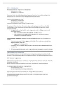
to be built of many small, interconnected subregions called elements. As an example
of how a finite element model might be used to represent a complex geometrical
shape, consider the milling machine structure. Since it is very difficult to find the
exact response (like stresses and displacements) of the machine under any specified
cutting (loading) condition, this structure is approximated as composed of several
pieces in the finite element method. In each piece or element, a convenient
approximate solution is assumed and the conditions of overall equilibrium of the
structure are derived. The satisfaction of these conditions will yield an approximate
solution for the displacements and stresses.
HISTORICAL BACKGROUND
Although the name of the finite element method was introduced in 1960 by Clough
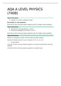
the concept dates back several centuries. For example, ancient mathematicians found
the circumference of a circle by approximating it by the perimeter of a polygon as
shown in Fig. 1.3. In terms of the present-day notation, each side of the polygon can
be called an element. By considering the approximating polygon inscribed or
,circumscribed, we can obtain a lower bound S(l) or an upper bound S(u) for the true
circumference S. Furthermore, as the number of sides of the polygon is increased,
the approximate values converge to the true value. These characteristics, as will be
seen later, will hold true in any general finite element application. To find the
differential equation of a surface of minimum area bounded by a specified closed
curve, in 1851 Schellback discretized the surface into several triangles and used a
finite difference expression to find the total discretized area [1.35]. In the current
finite element method, a differential equation is solved by replacing it by a set of
algebraic equations. Since the early 1900s, the behavior of structural frameworks,
composed of several bars arranged in a regular pattern, has been approximated by
that of an isotropic elastic body [1.36]. In 1943, Courant presented a method of
determining the torsional rigidity of a hollow shaft by dividing the cross section into
several triangles and using a linear variation of the stress function f over each triangle
in terms of the values of f at net points (called nodes in present-day finite element
terminology) [1.1]. This work is considered by some to be the origin of the present-
day finite element method. Since the Milling machine structure Finite element
idealization Arbor supports Arbor Cutter Table Column Overarm. Representation of
a milling machine structure by finite elements. Finite element mesh of a fighter
aircraft. Reprinted with permission from Anamet Laboratories, I Introduction mid-
1950s, engineers in the aircraft industry have worked on developing approximate
methods for the prediction of stresses induced in aircraft wings. In 1956, Turner et
al. [1.2] presented a method for modeling the wing skin using threenode triangles.
At about the same time, Argyris and Kelsey presented several papers outlining
matrix procedures, which contained some of the finite element ideas, for the solution
of structural analysis problems [1.3]. The study by Turner et al. [1.2] is considered
one of the key contributions in the development of the finite element method. The
name finite element was coined, for the first time, by Clough in 1960 [1.42].
,Although the finite element method was originally developed based mostly on
intuition and physical argument, the method was recognized as a form of the classic
Rayleigh-Ritz method in the early 1960s. Once the mathematical basis of the method
was recognized, the developments of new finite elements for different types of
problems and the popularity of the method started to grow almost exponentially
[1.37e1.40]. The digital computer provided a rapid means of performing the many
calculations involved in the finite element analysis (FEA) and made the method
practically viable. Along with the development of high-speed digital computers, the
application of the finite element method also progressed at a very impressive rate.
Zienkiewicz and his associates presented the broad interpretation of the method and
its applicability to any general field problem. The book by Przemieniecki presents
the finite element method as applied to the solution of stress analysis problems. With
this broad interpretation of the finite element method, it has been found that the finite
element equations can also be derived by using a weighted residual method such as
the Galerkin method or the least squares approach. This led to widespread interest
among applied mathematicians in applying the finite element method for the solution
of linear and nonlinear differential equations. Traditionally, mathematicians
developed techniques such as matrix theory and solution methods for differential
equations, and engineers used those methods to solve engineering analysis problems.
Only in the case of the finite element method, engineers developed and perfected the
technique; applied mathematicians use the method for the solution of complex
ordinary and partial differential equations. Today, it has become an industry standard
to solve practical engineering problems using the finite element method. Millions of
degrees of freedom (dof) are being used in the solution of some important practical
problems. Books that deal with the basic theory, mathematical foundations,
mechanical design, structural, fluid flow, heat transfer, electromagnetic and
manufacturing applications, and computer programming aspects are given at the end
, of the chapter [1.8e1.30]. The rapid progress of the finite element method can be
seen by noting that annually about 3800 papers were being published; a total of about
56,000 papers, 380 books, and 400 conference proceedings were published as
estimated in 1995 [1.40]. With all the progress, today the finite element method is
considered one of the well-established and convenient analysis tools by engineers
and applied scientists.
GENERAL APPLICABILITY OF THE METHOD
Although the method has been extensively used in the field of structural mechanics,
it has been successfully applied to solve several other types of engineering problems,
such as heat conduction, fluid dynamics, seepage flow, and electric and magnetic
fields. These applications prompted mathematicians to use this technique for the
solution of complicated boundary value and other problems. In fact, it has been
established that the method can be used for the numerical solution of ordinary and
partial differential equations. The general applicability of the finite element method
can be seen by observing the strong similarities that exist between various types of
engineering problems. For illustration, let us consider the following phenomena.
1.3.1 One-Dimensional Heat Transfer Consider the thermal equilibrium of an
element of a heated one-dimensional body as shown in Fig. 1.5A. The rate at which
heat enters the left face can be written as qx ¼ kA vT vx (1.1) where k is the thermal
conductivity of the material, A is the area of cross section through which heat flows
(measured perpendicular to the direction of heat flow), and vT/vx is the rate of
change of temperature T with respect to the axial direction The rate at which heat
leaves the right face can be expressed as (by retaining only two terms in the Taylor’s
series expansion) qxþdx ¼ qx þ vqx vx dx ¼ kA vT vx þ v vx kA vT vx dx (1.2)
The energy balance for the element for a small time dt is given by Heat inflow in
time dt þ Heat generated by internal sources in time dt ¼ Heat outflow in time dt þ
Change in internal energy during time dt That is, qxdt þ qA_ dx dt ¼ qxþdxdt þ cr
The basic idea in the finite element method is to find the solution of a complicated
problem by replacing it with a simpler one. Since the actual problem is replaced by
a simpler one in finding the solution, we will be able to find only an approximate
solution rather than the exact solution. The existing mathematical tools will not be
sufficient to find the exact solution (and sometimes, even an approximate solution)
of most of the practical problems. Thus, in the absence of any other convenient
method to find even the approximate solution of a given problem, we have to prefer
the finite element method. Moreover, in the finite element method, it will often be
possible to improve or refine the approximate solution by spending more
computational effort. In the finite element method, the solution region is considered
to be built of many small, interconnected subregions called elements. As an example
of how a finite element model might be used to represent a complex geometrical
shape, consider the milling machine structure. Since it is very difficult to find the
exact response (like stresses and displacements) of the machine under any specified
cutting (loading) condition, this structure is approximated as composed of several
pieces in the finite element method. In each piece or element, a convenient
approximate solution is assumed and the conditions of overall equilibrium of the
structure are derived. The satisfaction of these conditions will yield an approximate
solution for the displacements and stresses.
HISTORICAL BACKGROUND
Although the name of the finite element method was introduced in 1960 by Clough
the concept dates back several centuries. For example, ancient mathematicians found
the circumference of a circle by approximating it by the perimeter of a polygon as
shown in Fig. 1.3. In terms of the present-day notation, each side of the polygon can
be called an element. By considering the approximating polygon inscribed or
,circumscribed, we can obtain a lower bound S(l) or an upper bound S(u) for the true
circumference S. Furthermore, as the number of sides of the polygon is increased,
the approximate values converge to the true value. These characteristics, as will be
seen later, will hold true in any general finite element application. To find the
differential equation of a surface of minimum area bounded by a specified closed
curve, in 1851 Schellback discretized the surface into several triangles and used a
finite difference expression to find the total discretized area [1.35]. In the current
finite element method, a differential equation is solved by replacing it by a set of
algebraic equations. Since the early 1900s, the behavior of structural frameworks,
composed of several bars arranged in a regular pattern, has been approximated by
that of an isotropic elastic body [1.36]. In 1943, Courant presented a method of
determining the torsional rigidity of a hollow shaft by dividing the cross section into
several triangles and using a linear variation of the stress function f over each triangle
in terms of the values of f at net points (called nodes in present-day finite element
terminology) [1.1]. This work is considered by some to be the origin of the present-
day finite element method. Since the Milling machine structure Finite element
idealization Arbor supports Arbor Cutter Table Column Overarm. Representation of
a milling machine structure by finite elements. Finite element mesh of a fighter
aircraft. Reprinted with permission from Anamet Laboratories, I Introduction mid-
1950s, engineers in the aircraft industry have worked on developing approximate
methods for the prediction of stresses induced in aircraft wings. In 1956, Turner et
al. [1.2] presented a method for modeling the wing skin using threenode triangles.
At about the same time, Argyris and Kelsey presented several papers outlining
matrix procedures, which contained some of the finite element ideas, for the solution
of structural analysis problems [1.3]. The study by Turner et al. [1.2] is considered
one of the key contributions in the development of the finite element method. The
name finite element was coined, for the first time, by Clough in 1960 [1.42].
,Although the finite element method was originally developed based mostly on
intuition and physical argument, the method was recognized as a form of the classic
Rayleigh-Ritz method in the early 1960s. Once the mathematical basis of the method
was recognized, the developments of new finite elements for different types of
problems and the popularity of the method started to grow almost exponentially
[1.37e1.40]. The digital computer provided a rapid means of performing the many
calculations involved in the finite element analysis (FEA) and made the method
practically viable. Along with the development of high-speed digital computers, the
application of the finite element method also progressed at a very impressive rate.
Zienkiewicz and his associates presented the broad interpretation of the method and
its applicability to any general field problem. The book by Przemieniecki presents
the finite element method as applied to the solution of stress analysis problems. With
this broad interpretation of the finite element method, it has been found that the finite
element equations can also be derived by using a weighted residual method such as
the Galerkin method or the least squares approach. This led to widespread interest
among applied mathematicians in applying the finite element method for the solution
of linear and nonlinear differential equations. Traditionally, mathematicians
developed techniques such as matrix theory and solution methods for differential
equations, and engineers used those methods to solve engineering analysis problems.
Only in the case of the finite element method, engineers developed and perfected the
technique; applied mathematicians use the method for the solution of complex
ordinary and partial differential equations. Today, it has become an industry standard
to solve practical engineering problems using the finite element method. Millions of
degrees of freedom (dof) are being used in the solution of some important practical
problems. Books that deal with the basic theory, mathematical foundations,
mechanical design, structural, fluid flow, heat transfer, electromagnetic and
manufacturing applications, and computer programming aspects are given at the end
, of the chapter [1.8e1.30]. The rapid progress of the finite element method can be
seen by noting that annually about 3800 papers were being published; a total of about
56,000 papers, 380 books, and 400 conference proceedings were published as
estimated in 1995 [1.40]. With all the progress, today the finite element method is
considered one of the well-established and convenient analysis tools by engineers
and applied scientists.
GENERAL APPLICABILITY OF THE METHOD
Although the method has been extensively used in the field of structural mechanics,
it has been successfully applied to solve several other types of engineering problems,
such as heat conduction, fluid dynamics, seepage flow, and electric and magnetic
fields. These applications prompted mathematicians to use this technique for the
solution of complicated boundary value and other problems. In fact, it has been
established that the method can be used for the numerical solution of ordinary and
partial differential equations. The general applicability of the finite element method
can be seen by observing the strong similarities that exist between various types of
engineering problems. For illustration, let us consider the following phenomena.
1.3.1 One-Dimensional Heat Transfer Consider the thermal equilibrium of an
element of a heated one-dimensional body as shown in Fig. 1.5A. The rate at which
heat enters the left face can be written as qx ¼ kA vT vx (1.1) where k is the thermal
conductivity of the material, A is the area of cross section through which heat flows
(measured perpendicular to the direction of heat flow), and vT/vx is the rate of
change of temperature T with respect to the axial direction The rate at which heat
leaves the right face can be expressed as (by retaining only two terms in the Taylor’s
series expansion) qxþdx ¼ qx þ vqx vx dx ¼ kA vT vx þ v vx kA vT vx dx (1.2)
The energy balance for the element for a small time dt is given by Heat inflow in
time dt þ Heat generated by internal sources in time dt ¼ Heat outflow in time dt þ
Change in internal energy during time dt That is, qxdt þ qA_ dx dt ¼ qxþdxdt þ cr