ALC 9 Quantitative Research Techniques docs with complete solution
ALC 9 Quantitative Research Techniques docs with complete solution ALC 9 Quantitative Research Techniques docs -You take a random sample of 100 students at your university and find that their average GPA is 3.1. If you use this information to help you estimate the average GPA for all students at your university, then you are doing what branch of statistics? Descriptive statistics Inferential statistics Sample statistics Population statistics -A company has developed a new computer sound card whose average lifetime is unknown. In order to estimate this average, 200 sound cards are randomly selected from a large production line and tested; their average lifetime is found to be 5 years. The 200 sound cards represent a parameter. statistic. sample. population. -A company has developed a new computer sound card whose average lifetime is unknown. In order to estimate this average, 200 sound cards are randomly selected from a large production line and tested; their average lifetime is found to be 5 years. The five years represents a parameter. statistic. sample. population. -A summary measure that is computed from a population is called a sample. statistic. population. parameter. -Which of the following is a measure of the reliability of a statistical inference? A population parameter. A significance level. A descriptive statistic. A sample statistic. -The process of using sample statistics to draw conclusions about population parameters is called finding the significance level. calculating descriptive statistics. doing inferential statistics. calculating the confidence level. -Which of the following represents a population, as opposed to a sample? 1,000 respondents to a magazine survey which has 500,000 subscribers. The first 10 students in your class completing a final exam. Every fifth student to arrive at the book store on your campus. All registered voters in the State of Michigan. -A study in under way to determine the average height of all 32,000 adult pine trees in a certain national forest. The heights of 500 randomly selected adult pine trees are measured and analyzed. The sample in this study is the average height of the 500 randomly selected adult pine trees. the average height of all the adult pine trees in this forest. all adult pine trees in this forest. the 500 adult pine trees selected at random selected at random from this forest. -The significance level of a statistical inference measures the proportion of times a conclusion about a population will be correct in the long run. the proportion of times a conclusion about a population will be wrong in the long run. the proportion of times an estimation procedure will be correct in the long run. the proportion of times an estimation procedure will be wrong in the long run. -The confidence level of a statistical inference measures the proportion of times a conclusion about a population will be correct in the long run. the proportion of times a conclusion about a population will be wrong in the long run. the proportion of times an estimation procedure will be correct in the long run. the proportion of times an estimation procedure will be wrong in the long run. -A marketing research firm selects a random sample of adults and asks them a list of questions regarding their beverage preferences. What type of data collection is involved here? An experiment. A survey. Direct observation. None of these choices -Which of the following statements is true regarding the design of a good survey? The questions should be kept as short as possible. A mixture of dichotomous, multiple-choice, and open-ended questions may be used. Leading questions must be avoided. All of these choices are true. -Which method of data collection is involved when a researcher counts and records the number of students wearing backpacks on campus on a given day? An experiment. A survey. Direct observation. None of these choices. -The difference between a sample mean and the population mean is called nonresponse error. selection bias. sampling error. nonsampling error. -The manager of the customer service division of a major consumer electronics company is interested in determining whether the customers who have purchased a videocassette recorder over the past 12 months are satisfied with their products. If there are four different brands of videocassette recorders made by the company, the best sampling strategy would be to use a simple random sample. stratified random sample. cluster sample. self-selected sample. -When every possible sample with the same number of observations is equally likely to be chosen, the result is called a simple random sample. stratified random sample. cluster sample. biased sample. -Which of the following types of samples is almost always biased? Simple random samples. Stratified random samples. Cluster samples. Self-selected samples. -Which of the following is an example of a nonsampling error? Some incorrect responses are recorded. Responses are not obtained from all members of the sample. Some members of the target population cannot possibly be selected for the sample. All of these choices are true. -Which of the following situations lends itself to cluster samples? When it is difficult to develop a complete list of the population members. When the population members are widely disbursed. When selecting and collecting data from a simple random sample is too costly. All of these choices are true. -Which of the following causes sampling error? Taking a random sample from a population instead of studying the entire population. Making a mistake in the process of collecting the data. Nonresponse bias. All of these choices are true. -Which of the following describes selection bias? A leading question is selected for inclusion in the survey. Some members of the target population are excluded from possible selection for the sample. A person selected for the sample has a biased opinion about the survey. All of these choices are true. -An approach of assigning probabilities which assumes that all outcomes of the experiment are equally likely is referred to as the subjective approach. objective approach. classical approach. relative frequency approach. -The collection of all possible outcomes of an experiment is called a simple event. a sample space. a sample. a population. -If event A and event B cannot occur at the same time, then A and B are said to be mutually exclusive. independent. collectively exhaustive. None of these choices. -Which of the following best describes the concept of marginal probability? It is a measure of the likelihood that a particular event will occur, regardless of whether another event occurs. It is a measure of the likelihood that a particular event will occur, if another event has already occurred. It is a measure of the likelihood of the simultaneous occurrence of two or more events. None of these choices. -The intersection of events A and B is the event that occurs when either A or B occurs but not both. neither A nor B occur. both A and B occur. All of these choices are true. -If the outcome of event A is not affected by event B, then events A and B are said to be mutually exclusive. independent. collectively exhaustive. None of these choices. -Suppose P(A) = 0.35. The probability of the complement of A is 0.35. 0.65. -0.35 None of these choices. -If the events A and B are independent with P(A)=0.30 and P(B)=0.40, then the probability that both events will occur simultaneously is 0 0.12. 0.70. Not enough information to tell. -If A and B are mutually exclusive events with P(A) = 0.30 and P(B)=0.40, then P(A or B) is 0.10. 0.12. 0.70. None of these choices. -Bayes' Law is used to compute prior probabilities. joint probabilities. union probabilities. posterior probabilities. -Initial estimates of the probabilities of events are known as joint probabilities. posterior probabilities. prior probabilities. conditional probabilities. -The standard deviation of the sampling distribution of x̄ is also called the central limit theorem. standard error of the sample mean. finite population correction factor. population standard deviation -The Central Limit Theorem states that, if a random sample of size n is drawn from a population, then the sampling distribution of the sample mean is approximately normal if n > 30. is approximately normal if n < 30. is approximately normal if the underlying population is normal. None of these choices. -If all possible samples of size n are drawn from a population, the probability distribution of the sample mean x̄ is called the standard error of x̄. the expected value of x̄. the sampling distribution of x̄. he normal distribution. -Sampling distributions describe the distributions of population parameters. sample statistics. both parameters and statistics None of these choices. -Suppose X has a distribution that is not normal. The Central Limit Theorem is important in this case because t says the sampling distribution of x̄ is approximately normal for any sample size. it says the sampling distribution of x̄ is approximately normal if n is large enough. it says the sampling distribution of x̄ is exactly normal, for any sample size. None of these choices. -As a general rule, the normal distribution is used to approximate the sampling distribution of the sample proportion only if the sample size n is greater than 30. the population proportion p is close to 0.50. the underlying population is normal. np and n(1 - p) are both greater than or equal to 5. The standard deviation of p̂ is also called the standard error of the sample proportion. standard deviation of the population. standard deviation of the binomial. None of these choices. -If two populations are normally distributed, the sampling distribution of the difference in the sample means, x̄1 – x̄2 is approximately normal for any sample sizes. approximately normal if both sample sizes are large. exactly normal for any sample sizes. exactly normal only if both sample sizes are large. -If two random samples of sizes n1 and n2 are selected independently from two populations with means μ1 and μ2, then the mean of x̄1 - x̄2 equals μ1 + μ2 μ1 - μ2 μ1 / μ2 μ1 μ2 -If two random samples of sizes n1 and n2 are selected independently from two non-normally distributed populations, then the sampling distribution of the sample mean difference, x̄1 - x̄2 is always non-normal. is always normal. is approximately normal only if n1 and n2 are both larger than or equal to 30. is approximately normal regardless of n1 and n2. -The standard deviation of x̄1 - x̄2 is also called the standard error of the difference between two sample means. standard deviation of the difference between the population means. normal approximation to the difference of two binomial random variables. None of these choices. -The hypothesis of most interest to the researcher is the alternative hypothesis. the null hypothesis. both hypotheses are of equal interest. Neither hypothesis is of interest. - Type I error occurs when we reject a false null hypothesis. reject a true null hypothesis. don't reject a false null hypothesis. don't reject a true null hypothesis. -A Type II error is defined as rejecting a true null hypothesis. rejecting a false null hypothesis. not rejecting a true null hypothesis. not rejecting a false null hypothesis. -Which of the following probabilities is equal to the significance level α? Probability of making a Type I error. Probability of making a Type II error. Probability of rejecting H0 when you are supposed to. Probability of not rejecting H0 when you shouldn't. -If we reject the null hypothesis, we conclude that there is enough statistical evidence to infer that the alternative hypothesis is true. here is not enough statistical evidence to infer that the alternative hypothesis is true. there is enough statistical evidence to infer that the null hypothesis is true. there is not enough statistical evidence to infer that the null hypothesis is true. -Statisticians can translate p-values into several descriptive terms. Suppose you typically reject H0 at level 0.05. Which of the following statements is correct? If the p-value < 0.01, there is overwhelming evidence to infer that the alternative hypothesis is true. If 0.01 < p-value < 0.05, there is evidence to infer that the alternative hypothesis is true. If p-value > 0.10, there is no evidence to infer that the alternative hypothesis is true. All of these choices are true. -The p-value of a test is the smallest α at which the null hypothesis can be rejected. largest α at which the null hypothesis can be rejected. smallest α at which the null hypothesis cannot be rejected. largest α at which the null hypothesis cannot be rejected. -The numerical quantity computed from the data that is used in deciding whether to reject H0 is the significance level. critical value. test statistic. parameter. -For a given level of significance, if the sample size increases, the probability of a Type II error will remain the same. increase. decrease. be equal to 1.0 regardless of α. -The power of a test is measured by its capability of rejecting a null hypothesis that is true. not rejecting a null hypothesis that is true. rejecting a null hypothesis that is false. not rejecting a null hypothesis that is false. -If the probability of committing a Type I error for a given test is decreased, then for a fixed sample size n, the probability of committing a Type II error will decrease. increase. stay the same. Not enough information to tell. -A robust estimator is one that is unbiased and symmetrical about zero. consistent and is also mound-shaped. efficient and less spread out. not sensitive to moderate nonnormality. -For statistical inference about the mean of a single population when the population standard deviation is unknown, the degrees for freedom for the t-distribution equal n - 1 because we lose one degree of freedom by using the sample mean as an estimate of the population mean. sample standard deviation as an estimate of the population standard deviation. sample proportion as an estimate of the population proportion. sample size as an estimate of the population size. -The degrees of freedom for the test statistic for μ when σ is unknown is 1 n n - 1 None of these choices. -The statistic (n - 1)s2 / σ2 has a chi-squared distribution with n - 1 degrees of freedom if the population is normally distributed with variance equal to σ2 he sample is normally distributed with variance equal to s2. the sample has a Student t-distribution with degrees of freedom equal to n - 1. All of these choices are true. -Which of the following is an example illustrating the use of variance? As a measure of risk. As a judge of consistency. To search for and reduce variability in a process. All of these choices are true. -Which of the following conditions is needed regarding the chi-squared test statistic for the test of variance? The population random variable must be normal. The test statistic must be a non-negative number The test statistic must have a chi-squared distribution with n - 1 degrees of freedom. All of these choices are true. -Under what condition(s) does the test statistic for p have an approximate normal distribution? When np > 5. When np and np(1 - p) are both > 5. When n > 30. When np and n(1 - p) are both > 5. -In selecting the sample size to estimate the population proportion p, if we have no knowledge of even the approximate values of the sample proportion p̂ , we take another sample and estimate p̂ . we take two more samples and find the average of their p̂ let p̂ = 0.50. we let p̂ = 0.95. -When determining the sample size needed for a proportion for a given level of confidence and sampling error, the closer to 0.50 that p is estimated to be the smaller the sample size required. the larger the sample size required. he sample size is not affected. the effect cannot be determined from the information given. -Which of the following would be an appropriate null hypothesis? The population proportion is equal to 0.60. The sample proportion is equal to 0.60. The population proportion is not equal to 0.60. All of these choices are true. -The analysis of variance is a procedure that allows statisticians to compare two or more population means. proportions variances. standard deviations. -The distribution of the test statistic for analysis of variance is the normal distribution. Student t-distribution. F-distribution. None of these choices -In one-way analysis of variance, between-treatments variation is measured by the SSE SST SS(total) standard deviation. -When is the Tukey multiple comparison method used? To test for normality. To test equal variances. To test for equality of a group of population means. To test for differences in pairwise means. -In Fisher's least significant difference (LSD) multiple comparison method, the LSD value will be the same for all pairs of means if all sample means are the same. all sample sizes are the same. all population means are the same. None of these choices. -Fisher's least significant difference (LSD) multiple comparison method is flawed because it will increase α; the probability of committing a Type I error. it will increase β; the probability of committing a Type II error. it will increase both α and β, the probabilities of committing Type I and Type II errors, respectively. None of these choices. -When the objective is to compare more than two populations, the experimental design that is the counterpart of the matched pairs experiment is called a completely randomized design. one-way ANOVA design. randomized block design. None of these choices. -The primary interest of designing a randomized block experiment is to reduce the variation among blocks. increase the between-treatments variation to more easily detect differences among the treatment means. reduce the within-treatments variation to more easily detect differences among the treatment means None of these choices. -A complete 3 x 2 factorial experiment is called balanced if data is collected at all three levels of factor A. data is collected at both levels of factor B. the number of replicates is the same for each of the 6 treatments. None of these choices. -In a two-factor ANOVA, there are 4 levels for factor A, 5 levels for factor B, and 3 observations for each combination of factor A and factor B levels. The number of treatments in this experiment equals 60 25 20 16 -A tabular presentation that shows the outcome for each decision alternative under the various states of nature is called a payback period matrix. decision matrix. decision tree. payoff table. -Which of the following would be considered a state of nature for a business firm? Inventory levels Salaries for employees Site for new plant Worker safety laws -A payoff table lists the monetary values for each possible combination of the mean and median. mean and standard deviation. event (state of nature) and act (alternative). None of these choices. -Which of the following is true? The process of determining the EMV decision is called the rollback technique. We choose the act that produces the smallest expected opportunity loss (EOL). The EMV decision is always the same as the EOL decision. All of these choices are true. -Which of the following statements is false regarding the expected monetary value (EMV)? To calculate the EMV, the probabilities of the states of nature must be already decided upon. We choose the decision with the largest EMV. In general, the expected monetary values represent possible payoffs. None of these choices. -Which of the following statements is correct? The EMV criterion selects the act with the largest expected monetary value. The EOL criterion selects the act with the smallest expected opportunity loss. The expected value of perfect information (EVPI) equals the smallest expected opportunity loss. All of these choices are true. -The expected value of perfect information is the same as the expected monetary value for the best alternative. expected monetary value for the worst alternative. expected opportunity loss for the best alternative. expected opportunity loss for the worst alternative. -The expected value of sample information (EVSI) is the difference between the posterior probabilities and the prior probabilities of the states of nature. he expected payoff with perfect information (EPPI) and the expected monetary value for the best decision (EMV*). the expected monetary value with additional information (EMV') and the expected monetary value for the best decision (EMV*). the expected value of perfect information (EVPI) and the smallest expected opportunity loss (EOL*). -The procedure for revising probabilities based upon additional information is referred to as utility theory. Bernoulli's theorem. central limit theorem. Bayes' Law. -The difference between expected payoff under certainty and expected value of the best act without certainty is the expected monetary value. expected net present value. expected value of perfect information. expected rate of return. Quantitative Research Techniques What Is Statistics? What is Statistics “Statistics is a way to get information from data.” Statistics is a tool for creating new understanding from a set of numbers Descriptive Statistics A student enrolled in a business program is attending his first class of the required statistics course. The student is somewhat apprehensive because he believes the myth that the course is difficult. To alleviate his anxiety, the student asks the professor about last year's marks. Because, like all other statistics professors this one is friendly and helpful, he obliges the student and provides a list of the final marks, which are composed of term work plus the final exam. What information can the student obtain from the list? This is a typical statistics problem. The student has the data (marks) and needs to apply statistical techniques to get the information he requires. This is a function of descriptive statistics. Descriptive statistics deals with methods of organizing, summarizing, and presenting data in a convenient and informative way. One form of descriptive statistics uses graphical techniques, which allow statistics practitioners to present data in ways that make it easy for the reader to extract useful information. Another form of descriptive statistics uses numerical techniques to summarize data. One such method that you have already used frequently calculates the average or mean. In the same way that you calculate the average age of the employees of a company, we can compute the mean mark of last year's statistics course. The actual technique we use depends on what specific information we would like to extract. In this example, we can see at least three important pieces of information. The first is the "typical" mark. We call this a measure of central location. The average is one such measure. Suppose the student was told that the average mark last year was 67. Is this enough information to reduce his anxiety? The student would likely respond "no" because he would like to know whether most of the marks were close to 67 or were scattered far below and above the average. He needs a measure of variability. The simplest such measure is the range, which is calculated by subtracting the smallest number from the largest. Suppose the largest mark is 96 and the smallest is 24. Unfortunately, this provides little information. Moreover, the student must determine more about the marks. In particular he needs to know how the marks are distributed between 24 and 96. In the last few years, colleges and universities have signed exclusivity agreements with a variety of private companies. These agreements bind the university to sell that company's products exclusively on the campus. Many of the agreements involve food and beverage firms. A large university with a total enrollment of about 50,000 students has offered Pepsi-Cola an exclusivity agreement that would give Pepsi exclusive rights to sell its products at all university facilities for the next year with an option for future years. In return, the university would receive 35% of the on-campus revenues and an additional lump sum of $200,000 per year. Pepsi has been given 2 weeks to respond. The market for soft drinks is measured in terms of 12-ounce cans. Pepsi currently sells an average of 22,000 cans per week (over the 40 weeks of the year that the university operates). The cans sell for an average of 75 cents each. The costs including labor amount to 20 cents per can. Pepsi is unsure of its market share but suspects it is considerably less than 50%. A quick analysis reveals that if its current market share were 25%, then, with an exclusivity agreement, Pepsi would sell 88,000 (22,000 is 25% of 88,000) cans per week or 3,520,000 cans per year. The profit or loss can be calculated. The only problem is that we do not know how many soft drinks are sold weekly at the university. Pepsi assigned a recent university graduate to survey the university's students to supply the missing information. Accordingly, she organizes a survey that asks 500 students to keep track of the number of soft drinks they purchase in the next 7 days. The information we would like to acquire is an estimate of annual profits from the exclusivity agreement. The data are the numbers of cans of soft drinks consumed in 7 days by the 500 students in the sample. We can use descriptive techniques to learn more about the data. In this case, however, we are not so much interested in what the 500 students are reporting as we are in knowing the mean number of soft drinks consumed by all 50,000 students on campus. To accomplish this goal, we need another branch of statistics: inferential statistics. Inferential Statistics Inferential statistics is a body of methods used to draw conclusions or inferences about characteristics of populations based on sample data. The population in question in this case is the soft drink consumption of the university's 50,000 students. The cost of interviewing each student would be prohibitive and extremely time consuming. Statistical techniques make such endeavors unnecessary. Instead, we can sample a much smaller number of students (the sample size is 500) and infer from the data the number of soft drinks consumed by all 50,000 students. We can then estimate annual profits for Pepsi. When an election for political office takes place, the television networks cancel regular programming and instead provide election coverage. When the ballots are counted, the results are reported. However, for important offices such as president or senator in large states, the networks actively compete to see which will be the first to predict a winner. This is done through exit polls, wherein a random sample of voters who exit the polling booth is asked for whom they voted. From the data the sample proportion of voters supporting the candidates is computed. A statistical technique is applied to determine whether there is enough evidence to infer that the leading candidate will garner enough votes to win. The exit poll results from the state of Florida during the 2000 year elections were recorded (only the votes of the Republican candidate George W. Bush and the Democrat Albert Gore). The network analysts would like to know whether they can conclude that George W. Bush will win the state of Florida. Exit polls are a very common application of statistical inference. The population the television networks wanted to make inferences about is the approximately 5 million Floridians who voted for Bush or Gore for president. The sample consisted of the 765 people randomly selected by the polling company who voted for either of the two main candidates. The characteristic of the population that we would like to know is the proportion of the total electorate that voted for Bush. Specifically, we would like to know whether more than 50% of the electorate voted for Bush (counting only those who voted for either the Republican or Democratic candidate). Because we will not ask every one of the 5 million actual voters for whom they voted, we cannot predict the outcome with 100% certainty. A sample that is only a small fraction of the size of the population can lead to correct inferences only a certain percentage of the time. You will find that statistics practitioners can control that fraction and usually set it between 90% and 99%. Incidentally, on the night of the United States election in November 2000, the networks goofed badly. Using exit polls as well as the results of previous elections, all four networks concluded at 8:00 p.m. that Al Gore would win the state of Florida. Shortly after 10:00 p.m., the networks reversed course and declared that George W. Bush would win the state of Florida. By 2:00 a.m., another verdict was declared: The result was too close to call. Key Statistical Concepts Statistical inference problems involve three key concepts: the population, the sample, and the statistical inference. A population is the group of all items of interest to a statistics practitioner. It is frequently very large and may, in fact, be infinitely large. In the language of statistics, population does not necessarily refer to a group of people. It may, for example, refer to the population of diameters of ball bearings produced at a large plant. A descriptive measure of a population is called a parameter. In most applications of inferential statistics, the parameter represents the information we need. A sample is a set of data drawn from the population. A descriptive measure of a sample is called a statistic. We use statistics to make inferences about parameters. Statistical inference is the process of making an estimate, prediction, or decision about a population based on sample data. Because populations are almost always very large, investigating each member of the population would be impractical and expensive. It is far easier and cheaper to take a sample from the population of interest and draw conclusions or make estimates about the population on the basis of information provided by the sample. However, such conclusions and estimates are not always going to be correct. For this reason, we build into the statistical inference a measure of reliability. There are two such measures, the confidence level and the significance level. The confidence level is the proportion of times that an estimating procedure will be correct. When the purpose of the statistical inference is to draw a conclusion about a population, the significance level measures how frequently the conclusion will be wrong in the long run. Statistical inference is the process of making an estimate, prediction, or decision about a population based on a sample. What can we infer about a Population’s Parameters based on a Sample’s Statistics? Statistical Inference We use statistics to make inferences about parameters. Therefore, we can make an estimate, prediction, or decision about a population based on sample data. Thus, we can apply what we know about a sample to the larger population from which it was drawn! The rationale is large populations make investigating each member impractical and expensive. It is easier and cheaper to take a sample and make estimates about the population from the sample. However, such conclusions and estimates are not always going to be correct. For this reason, we build into the statistical inference “measures of reliability,” namely confidence level and significance level. The confidence level is the proportion of times that an estimating procedure will be correct. A confidence level of 95% means that estimates based on this form of statistical inference will be correct 95% of the time. When the purpose of the statistical inference is to draw a conclusion about a population, the significance level measures how frequently the conclusion will be wrong in the long run. A 5% significance level means that, in the long run, this type of conclusion will be wrong 5% of the time. Confidence and Significance Levels If we use α (Greek letter "alpha") to represent significance, then our confidence level is 1 - α This relationship can also be stated as: Confidence Level + Significance Level = 1 Consider a statement from polling data you may hear about in the news: "This poll is considered accurate within 3.4 percentage points, 19 times out of 20." In this case, our confidence level is 95% (19/20 = 0.95), while our significance level is 5%. A 5% significance level means, that in the long run, this type of conclusion will be wrong 5% of the time. Statistical analysis plays an important role in virtually all aspects of business and economics. Data Collection And Sampling Methods Of Collecting Data Statistics is a tool for converting data into information: But where then does data come from? How is it gathered? How do we ensure its accurate? Is the data reliable? Is it representative of the population from which it was drawn? The question arises: Where do data come from? The answer is that there are a large number of methods that produce data. Data are the observed values of a variable. That is, we define a variable or variables that are of interest to us and then proceed to collect observations of those variables. There are many methods used to collect or obtain data for statistical analysis. Three of the most popular methods are direct observation (number of customers entering a bank per hour), experiments (new ways to produce things to minimize costs), and surveys. The simplest method of obtaining data is by direct observation. When data are gathered in this way, they are said to be observational. For example, suppose that a researcher for a pharmaceutical company wants to determine whether aspirin does reduce the incidence of heart attacks. Observational data may be gathered by selecting a sample of men and women and asking each whether he or she has taken aspirin regularly over the past 2 years. Each person would be asked whether he or she had suffered a heart attack over the same period. The proportions reporting heart attacks would be compared and a statistical technique would be used to determine whether aspirin is effective in reducing the likelihood of heart attacks. There are many drawbacks to this method. One of the most critical is that it is difficult to produce useful information in this way. For example, if the statistics practitioner concludes that people who take aspirin suffer fewer heart attacks, can we conclude that aspirin is effective? It may be that people who take aspirin tend to be more health conscious, and health conscious people tend to have fewer heart attacks. The one advantage to direct observation is that it is relatively inexpensive. A more expensive but better way to produce data is through experiments. Data produced in this manner are called experimental. In the aspirin illustration, a statistics practitioner can randomly select men and women. The sample would be divided into two groups. One group would take aspirin regularly and the other would not. After 2 years, the statistics practitioner would determine the proportion of people in each group who had suffered a heart attack and again statistical methods would be used to determine whether aspirin works. If we find that the aspirin group suffered fewer heart attacks, we may more confidently conclude that taking aspirin regularly is a healthy decision. One of the most familiar methods of collecting data is the survey, which solicits information from people concerning such things as their income, family size, and opinions on various issues. The majority of surveys are conducted for private use. Private surveys are used extensively by market researchers to determine the preferences and attitudes of consumers and voters. An important aspect of surveys is the response rate. The response rate is the proportion of all people who were selected who complete the survey. A low response rate can destroy the validity of any conclusion resulting from the statistical analysis. Statistics practitioners need to ensure that data are reliable. Surveys Many researchers feel that the best way to survey people is by means of a personal interview, which involves an interviewer soliciting information from a respondent by asking prepared questions. A personal interview has the advantage of having a higher expected response rate than other methods of data collection. In addition, there will probably be fewer incorrect responses resulting from respondents misunderstanding some questions, because the interviewer can clarify misunderstandings when asked to. But the interviewer must also be careful not to say too much, for fear of biasing the response. The main disadvantage of personal interviews is that they are expensive, especially when travel is involved. A telephone interview is usually less expensive, but it is also less personal and has a lower expected response rate. Unless the issue is of interest, many people will refuse to respond to telephone surveys. This problem is exacerbated by telemarketers trying to sell something. Another popular method of data collection is the self-administered questionnaire, which is usually mailed to a sample of people. This is an inexpensive method of conducting a survey and is, therefore, attractive when the number of people to be surveyed is large. But self-administered questionnaires usually have a low response rate and may have a relatively high number of incorrect responses due to respondents misunderstanding some questions. Questionnaire Design Whether a questionnaire is self-administered or completed by an interviewer, it must be well designed. Proper questionnaire design takes knowledge, experience, time, and money. Over the years, a lot of thought has been put into the science of the design of survey questions. Key design principles include: Keep the questionnaire as short as possible. Most people are unwilling to spend much time filling out a questionnaire. Ask short, simple, and clearly worded questions to enable respondents to answer quickly, correctly, and without ambiguity. Start with demographic questions to help respondents get started and become comfortable quickly. Use dichotomous (yes|no) and multiple choice questions because of their simplicity. Use open-ended questions cautiously because they are time consuming and more difficult to tabulate and analyze. Avoid using leading questions that tend to lead the respondent to a particular answer. Pretest a questionnaire on a small number of people to uncover potential problems, such as ambiguous wording. Think about the way you intend to use the collected data when preparing the questionnaire. First determine whether you are soliciting values for an interval variable or a nominal variable. Then consider which type of statistical techniques, descriptive or inferential, you intend to apply to the data to be collected, and note the requirements of the specific techniques to be used. Sampling Recall that statistical inference permits us to draw conclusions about a population based on a sample. The chief motives for examining a sample rather than a population are cost and practicality. Statistical inference permits us to draw conclusions about a population parameter based on a sample that is quite small in comparison to the size of the population. It’s less expensive to sample 1,000 television viewers than 100 million TV viewers. Another illustration of sampling can be taken from the field of quality management. To ensure that a production process is operating properly, the operations manager needs to know what proportion of items being produced is defective. If the quality technician must destroy the item to determine whether it is defective, then there is no alternative to sampling: A complete inspection of the product population would destroy the entire output of the production process, which is impractical. The sample statistic can come quite close to the parameter it is designed to estimate if the target population (the population about which we want to draw inferences) and the sampled population (the actual population from which the sample has been taken) are the same. In practice, these may not be the same. In any case, the sampled population and the target population should be similar to one another. Self-selected samples are almost always biased, because the individuals who participate in them are more keenly interested in the issue than are the other members of the population. As a result, the conclusions drawn from such surveys are frequently wrong. Simple Random Sampling A sampling plan is just a method or procedure for specifying how a sample will be taken from a population. Three different sampling plans include simple random sampling, stratified random sampling, and cluster sampling. A simple random sample as seen in Figure 1 is a sample selected in such a way that every possible sample with the same number of observations is equally likely to be chosen. One way to conduct a simple random sample is to assign a number to each element in the population, write these numbers on individual slips of paper, toss them into a hat, and draw the required number of slips (the sample size, n) from the hat. This is the kind of procedure that occurs in raffles when all ticket stubs go into a large rotating drum from which the winners are selected. In making inferences about a population, we attempt to extract as much information as possible from a sample. The basic sampling plan, simple random sampling, often accomplishes this goal at low cost. Sometimes the elements of the population are already numbered such as Social Security numbers, employee numbers, or driver’s license numbers. In such cases, choosing which sampling procedure to use is simply a matter of deciding how to select from among these numbers. In other cases, the existing form of numbering has built-in flaws that make it inappropriate as a source of samples. Not everyone has a phone number, for example, so the telephone book does not list all the people in a given area. Couples often list the phone number under the man’s name, so telephone listings are likely to be disproportionately male. After each element of the chosen population has been assigned a unique number, sample numbers can be selected at random. A government income tax auditor must choose a sample of 40 of 1,000 returns to audit… A stratified random sample as seen in Figure 2 is obtained by separating the population into mutually exclusive sets, or strata, and then drawing simple random samples from each stratum. Examples of criteria for separating a population into strata (and of the strata themselves) include the following: Gender: male or female Age: under 20, 20-30, 31-40, 41-50, 51-60, over 60 Occupation: professional, clerical, blue-collar, other Household income: under $25,000; $25,000-$49,999; $50,000-$74,999; over $75,000 To illustrate, suppose a public opinion survey is to be conducted to determine how many people favor a tax increase. A stratified random sample could be obtained by selecting a random sample of people from each of the four income groups we just described. We usually stratify in a way that enables us to obtain particular kinds of information. In this example, we would like to know whether people in the different income categories differ in their opinions about the proposed tax increase, because the tax increase will affect the strata differently. We avoid stratifying when there is no connection between the survey and strata. For example, little purpose is served in trying to determine whether people within religious strata have divergent opinions about the tax increase. Stratified Random Sampling A stratified random sample is obtained by separating the population intomutually exclusive sets, or strata, and then drawing simple random samples from each stratum. We can acquire information about the total population, make inferences within a stratum, or make comparisons across strata. One advantage of stratification is that, besides acquiring information about the entire population, we can also make inferences within each stratum or compare strata. For instance, we can estimate what proportion of the lowest income group favors the tax increase, or we can compare the highest and lowest income groups to determine whether they differ in their support of the tax increase. Any stratification must be done in such a way that the strata are mutually exclusive: Each member of the population must be assigned to exactly one stratum. After the population has been stratified in this way, we can use simple random sampling to generate the complete sample. For example, we can draw random samples from each of the four income groups according to their proportions in the population. Thus, if in the population, the relative frequencies of the four groups are as listed in the chart in Figure 3, our sample will be stratified in the same proportions. If a total sample of 1,000 is to be drawn, we will randomly select 250 from stratum 1, 400 from stratum 2, 300 from stratum 3, and 50 from stratum 4. The problem with this approach, however, is that if we want to make inferences about the last stratum, a sample of 50 may be too small to produce useful information. In such cases, we usually increase the sample size of the smallest stratum to ensure that the sample data provide enough information for our purposes. An adjustment must then be made before we attempt to draw inferences about the entire population. After the population has been stratified, we can use simple random sampling to generate the complete sample: Cluster Sampling A cluster sample is a simple random sample of groups or clusters of elements versus a simple random sample of individual objects. Cluster sampling is particularly useful when it is difficult or costly to develop a complete list of the population members (making it difficult and costly to generate a simple random sample). It is also useful whenever the population elements are widely dispersed geographically. For example, suppose we wanted to estimate the average annual household income in a large city. To use simple random sampling, we would need a complete list of households in the city from which to sample. To use stratified random sampling, we would need the list of households, and we would also need to have each household categorized by some other variable (such as age of household head) in order to develop the strata. A less expensive alternative would be to let each block within the city represent a cluster. A sample of clusters could then be randomly selected, and every household within these clusters could be questioned to determine income. By reducing the distances the surveyor must cover to gather data, cluster sampling reduces the cost. But cluster sampling also increases sampling error, because households belonging to the same cluster are likely to be similar in many aspects, including household income. This can be partially offset by using some of the cost savings to choose a larger sample than would be used for a simple random sample. Whichever type of sampling plan you select, you still have to decide what size sample to use. We can rely on our intuition, which tells us that the larger the sample size is, the more accurate we can expect the sample estimates to be. Sampling Error Two major types of error can arise when a sample of observations is taken from a population: sampling error and non-sampling error. Anyone reviewing the results of sample surveys and studies, as well as statistics practitioners conducting surveys and applying statistical techniques, should understand the sources of these errors. Sampling error refers to differences between the sample and the population that exists only because of the observations that happened to be selected for the sample. Sampling error is an error that we expect to occur when we make a statement about a population that is based only on the observations contained in a sample taken from the population. To illustrate, suppose that we wish to determine the mean annual income of North American blue-collar workers. To determine this parameter, we would have to ask each North American blue-collar worker what his or her income is and then calculate the mean of all the responses. Because the size of this population is several million, the task is both expensive and impractical. We can use statistical inference to estimate the mean income of the population if we are willing to accept less than 100% accuracy. We record the incomes of a sample of the workers and find the mean xÌ„ of this sample of incomes. This sample mean is an estimate of the desired population mean. But the value of the sample mean will deviate from the population mean simply by chance, because the value of the sample mean depends on which incomes just happened to be selected for the sample. he difference between the true (unknown) value of the population mean and its estimate, the sample mean, is the sampling error. The size of this deviation may be large simply due to bad luck - bad luck that a particularly unrepresentative sample happened to be selected. The only way we can reduce the expected size of this error is to take a larger sample. Given a fixed sample size, the best we can do is to state the probability that the sampling error is less than a certain amount. It is common today for such a statement to accompany the results of an opinion poll. If an opinion poll states that, based on sample results, the incumbent candidate for mayor has the support of 54% of eligible voters in an upcoming election, the statement may be accompanied by the following explanatory note: This percentage is correct to within three percentage points, 19 times out of 20. This statement means that we estimate that the actual level of support for the candidate is between 51% and 57%; and that in the long run, this type of procedure is correct 95% of the time. Nonsampling Errors Nonsampling error is more serious than sampling error, because taking a larger sample won't diminish the size, or the possibility of occurrence, of this error. Even a census can (and probably will) contain nonsampling errors. Nonsampling errors are due to mistakes made in the acquisition of data or due to the sample observations being selected improperly. Three types of nonsampling errors are errors in data acquisition, nonresponse errors, and selection bias. Errors in data acquisition arise from the recording of incorrect responses. Incorrect responses may be the result of incorrect measurements being taken because of faulty equipment, mistakes made during transcription from primary sources, inaccurate recording of data due to misinterpretation of terms, or inaccurate responses to questions concerning sensitive issues such as sexual activity or possible tax evasion. Nonresponse error refers to error (or bias) introduced when responses are not obtained from some members of the sample. When this happens, the sample observations that are collected may not be representative of the target population, resulting in biased results. The response rate, the proportion of all people selected who complete the survey, is a key survey parameter and helps in the understanding in the validity of the survey and sources of nonresponse error. Nonresponse can occur for a number of reasons. An interviewer may be unable to contact a person listed in the sample, or the sampled person may refuse to respond for some reason. In either case, responses are not obtained from a sampled person, and bias is introduced. The problem of nonresponse is even greater when self-administered questionnaires are used rather than an interviewer, who can attempt to reduce the nonresponse rate by means of callbacks. The Literary Digest was a popular magazine is the 1920s and 1930s that had correctly predicted the outcomes of several presidential elections. In 1936, the Literary Digest predicted that Alfred Landon would defeat Franklin D. Roosevelt. But in that election, Roosevelt defeated Landon in a landslide victory, garnering the support of 62% of the electorate. The Literary Digest sent out 10 million sample ballots to prospective voters. However, most of the names of these people were taken from the Digest’s subscription list and from telephone directories. Only 2.3 million ballots were returned, which was a high nonresponse rate, resulting in a biased, self-selected sample. Selection bias occurs when the sampling plan is such that some members of the target population cannot possibly be selected for inclusion in the sample. Together with nonresponse error, selection bias played a role in the Literary Digest poll being so wrong, as voters without telephones or without a subscription to Literary Digest were excluded from possible inclusion in the sample taken. Probability Assigning Probability To Events To introduce probability, we must first define a random experiment. A random experiment is an action or process that leads to one of several possible outcomes. Here are six illustrations of random experiments and their outcomes. Illustration 1. Experiment: Outcomes: Illustration 2. Experiment: Outcomes: Illustration 3. Experiment: Outcomes: Illustration 4. Experiment: Outcomes: Illustration 5. Experiment: Outcomes: Illustration 6. Experiment: Flip a coin. Heads and tails Record marks on a statistics test (out of 100). Numbers between 0 and 100 Record grade on a statistics test. A, B, C, D, and F Record student evaluations of a course. Poor, fair, good, very good, and excellent Measure the time to assemble a computer. Number whose smallest possible value is 0 seconds with no predefined upper limit Record the party that a voter will vote for in an upcoming election. Outcomes: Party A, Party B,… Requirements of Probability The first step in assigning probabilities is to produce a list of the outcomes. The listed outcomes must be exhaustive, which means that all possible outcomes must be included. Additionally, the outcomes must be mutually exclusive, which means that no two outcomes can occur at the same time. A list of exhaustive and mutually exclusive outcomes is called a sample space and is denoted by S. The outcomes are denoted by O1, O2,..., Ok. A sample space of a random experiment is a list of all possible outcomes of the experiment. The outcomes must be exhaustive and mutually exclusive. Using set notation we represent the sample space and its outcomes as S = {O1, O2,..., Ok} Once a sample space has been prepared, we begin the task of assigning probabilities to the outcomes. There are three ways to assign probability to outcomes. However it is done, there are two rules governing probabilities. The probability of any outcome must lie between 0 and 1. That is,0 ≤ P(Oi) ≤ 1 for each i Note: P(Oi) is the notation we use to represent the probability of outcome i. The sum of the probabilities of all the outcomes in a sample space must be 1. That is, Σ ki=1 P(Oi) = 1 Three Approaches of Assigning Probability The classical approach is used by mathematicians to help determine probability associated with games of chance. If an experiment has n possible outcomes, this method would assign a probability of 1/n to each outcome. For example, the classical approach specifics that the probabilities of heads and tails in the flip of a balanced coin are equal to each other. Because the sum of the probabilities must be 1, the probability of heads and the probability of tails are both 50%. Similarly, the six possible outcomes of the toss of a balanced die have the same probability; each is assigned a probability of 1/6. In some experiments it is necessary to develop mathematical ways to count the number of outcomes. Figure 1 shows the classical approach when rolling two dice. Figure 1: Classical Approach Experiment: Rolling two dice and observing the total Outcomes: {2, 3, ..., 12} Examples: The relative frequency approach defines probability as the long-run relative frequency with which an outcome occurs. For example, suppose that we know that of the last 1,000 students who took the statistics course you’re now taking, 200 received a grade of A. The relative frequency of A’s is then 200/1000 or 20%. This figure represents an estimate of the probability of obtaining a grade of A in the course. It is only an estimate because the relative frequency approach defines probability as the “long-run” relative frequency. One thousand students do not constitute the long run. The larger the number of students whose grades we have observed, the better the estimate becomes. In theory we would have to observe an infinite number of grades to determine the exact probability. Figure 2 and Figure 3 shows the relative frequency approach used by Bits & Bytes Computer Shop to construct the probabilities that the shop will sell a certain number of desktop computer systems on a given day. When it is not reasonable to use the classical approach and there is no history of the outcomes, we have no alternative but to employ the subjective approach. In the subjective approach, we define probability as the degree of belief that we hold in the occurrence of an event. An excellent example is derived from the field of investment. An investor would like to know the probability that a particular stock will increase in value. Using the subjective approach, the investor would analyze a number of factors associated with the stock and the stock market in general and, using his or her judgment, assign a probability to the outcomes of interest. Weather forecasting’s “P.O.P.” is another example of the subjective approach. “Probability of Precipitation” (P.O.P.) is defined in different ways by different forecasters, but basically it’s a subjective probability based on past observations combined with current weather conditions. A P.O.P. of 60% means that based on current conditions, there is a 60% chance of rain. Interpreting Probability No matter which method is used to assign probability, we interpret it using the relative frequency approach for an infinite number of experiments. For example, an investor may have used the subjective approach to determine that there is a 65% probability that a particular stock’s price will increase over the next month. However, we interpret the 65% figure to mean that if we had an infinite number of stocks with exactly the same economic and market characteristics as the one the investor will buy, 65% of them will increase in price over the next month. Similarly, we can determine that the probability of throwing a 5 with a balanced die is 1/6. We may have used the classical approach to determine this probability. However, we interpret the number as the proportion of times that a 5 is observed on a balanced die thrown an infinite number of times. Another example would be a government lottery game where 6 numbers (of 49) are picked. The classical approach would predict the probability for any one number being picked as 1/49 = 2.04%. We interpret this to mean that in the long run, each number will be picked 2.04% of the time. This relative frequency approach is useful to interpret probability statements such as those heard from weather forecasters or scientists. You will also discover that this is the way we link the population and the sample in statistical inference. Joint Probability We will now discuss how to calculate the probability of more complicated events from the probability of related events. Here is an illustration of the process. The sample space for the toss of a die is S = {1,2,3,4,5,6}. If the die is balanced, the probability of each simple event is 1/6. In most parlor games and casinos, players toss two dice. To determine playing and wagering strategies, players need to compute the probabilities of various totals of the two dice. For example, the probability of tossing a total of 3 with two dice is 2/36. This probability was derived by creating combinations of the simple events. Once of the most important types is the intersection of two events. The intersection of events A and B is the event as seen in Figure 4 that occurs when both A and B occur. It is denoted as A and B. The probability of the intersection is called the joint probability. For example, one way to toss a 3 with two dice is to toss a 1 on the first die and a 2 on the second die, which is the intersection of two simple events. Incidentally, to compute the probability of a total of 3, we need to combine this intersection with another intersection, namely, a 2 on the first die and a 1 on the second die. This type of combination is called a union of two events as seen in Figure 5. It is denoted as A or B. The table in Figure 6 tells us that the joint probability that a mutual fund outperforms the market and that its manager graduated from a top-20 MBA program is .11. That is, 11% of all mutual funds outperform the market and their managers graduated from a top-20 MBA program. The other three joint probabilities are defined similarly. That is, the probability that a mutual fund outperforms the market and its manager did not graduate from a top-20 MBA program is .06. The probability that a mutual fund does not outperform the market and its manager graduated from a top-20 MBA program is .29. The probability that a mutual fund does not outperform the market and its manager did not graduate from a top-20 MBA program is .54. To help make our task easier, we'll use notation to represent the events. Let A1 = Fund manager graduated from a top-20 MBA program A2 = Fund manager did not graduate from a top-20 MBA program B1 = Fund outperforms the market B2 = Fund does not outperform the market Thus, P(A1 and B1) = .11 P(A2 and B1) = .06 P(A1 and B2) = .29 P(A2 and B2) = .54 Marginal Probability The joint probabilities allow us to compute various probabilities. Marginal probability is a measure of the likelihood that a particular event will occur, regardless of whether another event occurs. Marginal probabilities, computed by adding across rows or down columns, are so named because they are calculated in the margins of the table as seen in Figure 7. Adding across the first row produces P(A1 and B1) + P(A1 and B2) = .11 + .29 = .40. Notice that both intersections state that the manager graduated from a top-20 MBA program (represented by A1). Thus, when randomly selecting mutual funds, the probability that its manager graduated from a top-20 MBA program is .40. Expressed as relative frequency, 40% of all mutual fund managers graduated from a top-20 MBA program. Adding across the second row produces P(A2 and B1) + P(A2 and B2) = .06 + .54 = .60. This probability tells us that 60% of all mutual fund managers did not graduate from a top-20 MBA program (represented by A2). Notice that the probability that a mutual fund manager graduated from a top-20 MBA program and the probability that the manager did not graduate from a top-20 MBA program add to 1. Adding down the columns produces the following marginal probabilities.: Column 1: P(A1 and B1) + P(A2 and B1) = .11 + .06 = .17 Column 2: P(A1 and B2) + P(A2 and B2) = .29 + .54 = .83 These marginal probabilities tell us that 17% of all mutual funds outperform the market and that 83% of mutual funds do not outperform the market. Conditional Probability We frequently need to know how two events are related. Conditional probability is used to determine how two events are related; that is, we can determine the probability of one event given the occurrence of another related event. For example, we would certainly like to know the probability that a fund managed by a graduate of a top-20 MBA program will outperform the market. Such a probability will allow us to make an informed decision about where to invest our money. This probability is called a conditional probability because we want to know the probability that a fund will outperform the market given the condition that the manager graduated from a top-20 MBA program. Conditional probabilities are written as P(A | B) and read as “ the probability of A given B” and is calculated as P(A | B) =
École, étude et sujet
- Établissement
- ALC EXAMS
- Cours
- ALC EXAMS
Infos sur le Document
- Publié le
- 6 décembre 2021
- Nombre de pages
- 54
- Écrit en
- 2021/2022
- Type
- Examen
- Contient
- Questions et réponses
Sujets
-
alc 9 quantitative research techniques docs
-
you take a random sample of 100 students at your university and find that their average gpa is 31 if you use this information to help you estimate the ave
Document également disponible en groupe