Standard regression analysis (SRA)
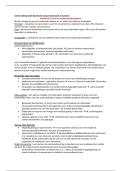
Linear regression analysis
- Describes relationship by fitting line to observed data.
- Uses straight line (logistic/non-linear models use a curved line).
- Estimating how dependent variable changes as independent variable(s) change.
- Y = predicted value dependent for any given value of the independent variable
- B0 = intercept
Predicted value Y when X = 0
- B1 = regression coefficient
How much Y changes as X increases
Denotes magnitude of change in Y
- X = independent variable
- E = error of the estimate
The amount of variation in the estimate of the regression coefficient
OBTAINING REGRESSION LINE
- Least square means = finding best fit for data set points by minimizing the sum of residuals of
points from the plotted curve.
3 steps:
1. Square each residual
2. Sum all squared residuals
3. Minimize the total of the squared values
ASSUMPTIONS
1. Linear relationship between X and Y
2. Normal distribution residuals
3. Homoscedasticity residuals
4. Independent observations
- Independent-samples T-test = to compare means between 2 unrelated groups on the same
continuous Y.
- One-way ANOVA = to compare means between >3 unrelated groups on the same continuous Y.
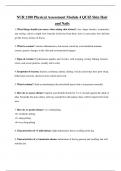
LINEAR REGRESSION ANALYSIS OUTCOME
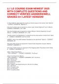
,Logistic regression analysis
- Describes relationship between binary Y and >1 other covariates (X).
- To fit a line between observations Y is transformed into the logarithm of the odds (ln(odds)).
- E-power of b1 = odds ratio (Exp(B)).
- Ln(odds of …) = the natural log of the odds of the outcome
- B0 = intercept
The natural log of the odds of the outcome when X = 0
- B1 = regression coefficient
How much ln(odds of …) changes when X changes with 1 unit
taking the E-power of b1 gives the odds ratio (more easy to interpret)
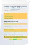
LOGISTIC REGRESSION ANALYSIS OUTCOME
Confounding
- Confounding = a distortion that modifies an relationship between exposure and outcome, because
the factor is associated with both exposure and outcome.
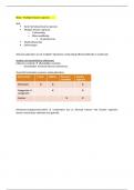
- Re-assess b1 after adding the potential confounder (b2) into the model.
compare crude b1 and adjusted b1 and calculate the percentage difference in the b1
Crude b1 Adjusted b1
Logistic -0.461 -0.388
Linear 2.149 2.212
Calculation logistic
-0.% = -0.00461
1% = -0.00461
-0.388 / -0.00461 = 84
100 – 84 = 16% >10% there is confounding by
sex
Calculation linear
2.% = 0.02149
1% = 0.02149
2..02149 = 102.9
100 – 102.9 = -2.9% <10% there is no confounding by sex
,Effect modification
- Effect modification = when magnitude of effect exposure (X) on Y differs between the level of the
third variable.
exposure having different effects
- Assess p-value of interaction term (third variable).
- If significant, results of effect should be reported separately for the different subgroups.
,Basic principles linear mixed model
analysis
- Linear MMA extended version of linear regression analysis.
- Clustering is present when a set of objects group in such a way that objects in the same group (=
cluster) are more similar to each other than to those in other clusters.
- Observations within clusters are correlated with each other.
- You have to take this into account in your analysis with MMA.
Similar approach in regression models with clustering:
1. Intercept (u)
2. Slope (uk)
3. Intercept and slope (ukj)
General idea MMA – 3 steps
1. Estimate intercepts(/slopes) for different groups
2. Draw a normal distribution over the different intercepts(/slopes)
3. Estimate the variance of that normal distribution
Covariance between random slope & random
intercept
- Also known as the covariance (interaction) between the random slope and
random intercept.
1. Negative covariance
Indicates inverse relationship
For levels with relatively high intercept, a relatively low slope is observed
2. Positive covariance
Indicates same relationship
4. For levels with relatively high intercept, a relatively high slope is observed
Intraclass Correlation Coefficient (ICC) – ICC as
indicator
- ICC = indication average correlation of observations of subjects living in the same cluster.
- Indicates how strong units in the same group resemble each other (correlation).
- When calculating ICC with a model that includes an X variable, remaining variance is lower.
- Pure ICC calculated with intercept-only model (model without X).
,Variance used as explanation (specific application MMA)
- Using random effects for explanation differences.
- % of the difference in Y between the levels of the cluster is explained by X.
- Calculate with random intercept of the intercept-only model and the random intercept of the
model with X.
, Example linear MM
Explained with cross-sectional cohort study investigating the relationship between X (physical activity = PA)
and Y (health).
- Two-level structure
Subject = lowest level
Neighbourhood (NBH) = highest level
- Linear regression analysis should adjust for NBH by MMA.
1. Naïve linear MMA
- Without an adjustment for NBH
General information
- MMA without adjustment
- Log likelihood
- Number of observations
Fixed part
- Activity = b1, with standard error (S.E.), z-value, corresponding p-value and 95% CI estimated
around the b1.
Difference in health when there is 1 unit difference in PA
- _cons = intercept
Value of health when PA equals 0
Random part
- Var(Residual) = residual variance (the error variance/unexplained variance).
Because it’s a naïve model, random part only contains variance of the residual.
2. Add random intercept to the model
- Adding a random intercept on cluster level to the model.
- To adjust for NBH level.
Linear regression analysis
- Describes relationship by fitting line to observed data.
- Uses straight line (logistic/non-linear models use a curved line).
- Estimating how dependent variable changes as independent variable(s) change.
- Y = predicted value dependent for any given value of the independent variable
- B0 = intercept
Predicted value Y when X = 0
- B1 = regression coefficient
How much Y changes as X increases
Denotes magnitude of change in Y
- X = independent variable
- E = error of the estimate
The amount of variation in the estimate of the regression coefficient
OBTAINING REGRESSION LINE
- Least square means = finding best fit for data set points by minimizing the sum of residuals of
points from the plotted curve.
3 steps:
1. Square each residual
2. Sum all squared residuals
3. Minimize the total of the squared values
ASSUMPTIONS
1. Linear relationship between X and Y
2. Normal distribution residuals
3. Homoscedasticity residuals
4. Independent observations
- Independent-samples T-test = to compare means between 2 unrelated groups on the same
continuous Y.
- One-way ANOVA = to compare means between >3 unrelated groups on the same continuous Y.
LINEAR REGRESSION ANALYSIS OUTCOME
,Logistic regression analysis
- Describes relationship between binary Y and >1 other covariates (X).
- To fit a line between observations Y is transformed into the logarithm of the odds (ln(odds)).
- E-power of b1 = odds ratio (Exp(B)).
- Ln(odds of …) = the natural log of the odds of the outcome
- B0 = intercept
The natural log of the odds of the outcome when X = 0
- B1 = regression coefficient
How much ln(odds of …) changes when X changes with 1 unit
taking the E-power of b1 gives the odds ratio (more easy to interpret)
LOGISTIC REGRESSION ANALYSIS OUTCOME
Confounding
- Confounding = a distortion that modifies an relationship between exposure and outcome, because
the factor is associated with both exposure and outcome.
- Re-assess b1 after adding the potential confounder (b2) into the model.
compare crude b1 and adjusted b1 and calculate the percentage difference in the b1
Crude b1 Adjusted b1
Logistic -0.461 -0.388
Linear 2.149 2.212
Calculation logistic
-0.% = -0.00461
1% = -0.00461
-0.388 / -0.00461 = 84
100 – 84 = 16% >10% there is confounding by
sex
Calculation linear
2.% = 0.02149
1% = 0.02149
2..02149 = 102.9
100 – 102.9 = -2.9% <10% there is no confounding by sex
,Effect modification
- Effect modification = when magnitude of effect exposure (X) on Y differs between the level of the
third variable.
exposure having different effects
- Assess p-value of interaction term (third variable).
- If significant, results of effect should be reported separately for the different subgroups.
,Basic principles linear mixed model
analysis
- Linear MMA extended version of linear regression analysis.
- Clustering is present when a set of objects group in such a way that objects in the same group (=
cluster) are more similar to each other than to those in other clusters.
- Observations within clusters are correlated with each other.
- You have to take this into account in your analysis with MMA.
Similar approach in regression models with clustering:
1. Intercept (u)
2. Slope (uk)
3. Intercept and slope (ukj)
General idea MMA – 3 steps
1. Estimate intercepts(/slopes) for different groups
2. Draw a normal distribution over the different intercepts(/slopes)
3. Estimate the variance of that normal distribution
Covariance between random slope & random
intercept
- Also known as the covariance (interaction) between the random slope and
random intercept.
1. Negative covariance
Indicates inverse relationship
For levels with relatively high intercept, a relatively low slope is observed
2. Positive covariance
Indicates same relationship
4. For levels with relatively high intercept, a relatively high slope is observed
Intraclass Correlation Coefficient (ICC) – ICC as
indicator
- ICC = indication average correlation of observations of subjects living in the same cluster.
- Indicates how strong units in the same group resemble each other (correlation).
- When calculating ICC with a model that includes an X variable, remaining variance is lower.
- Pure ICC calculated with intercept-only model (model without X).
,Variance used as explanation (specific application MMA)
- Using random effects for explanation differences.
- % of the difference in Y between the levels of the cluster is explained by X.
- Calculate with random intercept of the intercept-only model and the random intercept of the
model with X.
, Example linear MM
Explained with cross-sectional cohort study investigating the relationship between X (physical activity = PA)
and Y (health).
- Two-level structure
Subject = lowest level
Neighbourhood (NBH) = highest level
- Linear regression analysis should adjust for NBH by MMA.
1. Naïve linear MMA
- Without an adjustment for NBH
General information
- MMA without adjustment
- Log likelihood
- Number of observations
Fixed part
- Activity = b1, with standard error (S.E.), z-value, corresponding p-value and 95% CI estimated
around the b1.
Difference in health when there is 1 unit difference in PA
- _cons = intercept
Value of health when PA equals 0
Random part
- Var(Residual) = residual variance (the error variance/unexplained variance).
Because it’s a naïve model, random part only contains variance of the residual.
2. Add random intercept to the model
- Adding a random intercept on cluster level to the model.
- To adjust for NBH level.