Summary Research Toolbox
What is important in design?
- Safety
- Efficiency / effectivity
- Comfort
- Esthetics
Recall is higher during mouse-tracking, may be caused by:
- Pt.’s spend more time viewing
- Pt.’s are more aware of the task
Sampling & compression
Frequency how many times a waves repeats in 1 sec
Problems with sampling:
- Aliasing: when a high freq looks like a low freq after
sampling because of a too low sampling frequency
o Avoided using Nyquist frequency (highest freq that
you can capure) sampling frequency should be
twice the Nyquist freq
o E.g. CD’s are twice the freq (44 KHz) of what humans
can max. hear (20 KHz)
o Moiré patterns: a weird pattern that appears when
aliasing happens to a fine pattern
- Limited throughput of computers cannot handle too big
files. Solutions:
o Count colors, them adjust bit depth to minimum
amount of colors that you want coded
o Produce image to target resolution (screen that is
used) it’s a waste to make images with higher res
when they can’t be displayed properly
o Use compression reduce file size by smartly
encoding information. 2 types:
Lossy (e.g. jpg, mp3)
Pro: effective way of compressing, file
becomes really small.
Con: relevant details get lost.
Lossless (e.g. zip, png, flac)
Pro: details are preserved, no relevant info
gets lost.
, Con: files can still be big
Prospect theory loss feels worse than how happy the same
amount of gain makes you feel.
Relatively, people like small gain over big gain.
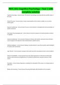
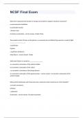
Signal detection theory (SDT)
Z / prevalence ~Z
PPV False pos / FA
True pos / hits
True neg /
correct rejections
False neg / misses
NPV
Disease z:
hits+ misses
Prevalence / prior p(z):
z
z+ z
, No disease ~z:
FA+c orrect rejection s
Posterior / positive predictive value (PPV): the chance that you
have the disease when you tested positive (i.e. that it is not a
false alarm):
p¿
Sensitivity / hit-rate: the chance that you test positive when you
have the disease (i.e. that it is not a miss)
hits true pos
p ( +¿ z )=
z =hits+misses = true pos+ false ¬¿ ¿
Specificity / CR-rate: chance that you test negative when you
don’t have the disease (i.e. that it is not a false alarm):
correct rejections ¬¿
p (−¿ z )= =true ¿
z =FA +correct rejection s false pos +true ¬¿ ¿
Odds
Odds range from 0 to ∞ (e.g. 1:3), while probs range from 0 to 1
(e.g. 1/4).
Transforming:
p
- Odds to probs: Ω= 1−p =
Ω
- Probs to odds: p ¿ 1+ Ω
Bayes’ rule in odds
hit −rate prevalence
= FA−rate 1−prevalence
Likelihood ratio = Bayes factor (hits/FA) = diagnostic value (for
‘yes’)
What is important in design?
- Safety
- Efficiency / effectivity
- Comfort
- Esthetics
Recall is higher during mouse-tracking, may be caused by:
- Pt.’s spend more time viewing
- Pt.’s are more aware of the task
Sampling & compression
Frequency how many times a waves repeats in 1 sec
Problems with sampling:
- Aliasing: when a high freq looks like a low freq after
sampling because of a too low sampling frequency
o Avoided using Nyquist frequency (highest freq that
you can capure) sampling frequency should be
twice the Nyquist freq
o E.g. CD’s are twice the freq (44 KHz) of what humans
can max. hear (20 KHz)
o Moiré patterns: a weird pattern that appears when
aliasing happens to a fine pattern
- Limited throughput of computers cannot handle too big
files. Solutions:
o Count colors, them adjust bit depth to minimum
amount of colors that you want coded
o Produce image to target resolution (screen that is
used) it’s a waste to make images with higher res
when they can’t be displayed properly
o Use compression reduce file size by smartly
encoding information. 2 types:
Lossy (e.g. jpg, mp3)
Pro: effective way of compressing, file
becomes really small.
Con: relevant details get lost.
Lossless (e.g. zip, png, flac)
Pro: details are preserved, no relevant info
gets lost.
, Con: files can still be big
Prospect theory loss feels worse than how happy the same
amount of gain makes you feel.
Relatively, people like small gain over big gain.
Signal detection theory (SDT)
Z / prevalence ~Z
PPV False pos / FA
True pos / hits
True neg /
correct rejections
False neg / misses
NPV
Disease z:
hits+ misses
Prevalence / prior p(z):
z
z+ z
, No disease ~z:
FA+c orrect rejection s
Posterior / positive predictive value (PPV): the chance that you
have the disease when you tested positive (i.e. that it is not a
false alarm):
p¿
Sensitivity / hit-rate: the chance that you test positive when you
have the disease (i.e. that it is not a miss)
hits true pos
p ( +¿ z )=
z =hits+misses = true pos+ false ¬¿ ¿
Specificity / CR-rate: chance that you test negative when you
don’t have the disease (i.e. that it is not a false alarm):
correct rejections ¬¿
p (−¿ z )= =true ¿
z =FA +correct rejection s false pos +true ¬¿ ¿
Odds
Odds range from 0 to ∞ (e.g. 1:3), while probs range from 0 to 1
(e.g. 1/4).
Transforming:
p
- Odds to probs: Ω= 1−p =
Ω
- Probs to odds: p ¿ 1+ Ω
Bayes’ rule in odds
hit −rate prevalence
= FA−rate 1−prevalence
Likelihood ratio = Bayes factor (hits/FA) = diagnostic value (for
‘yes’)