MANAGERIALECONOMICS
SimonKuhn
LECTURE1:FOUNDATIONS
PARTONE
WHATISINDUSTRIALORGANISATION?
IndustrialOrganisationisabranchofeconomicsthatisconcernedwiththestudyofimperfect
competition.Wewilllookatwaysforacompanytoescapeperfectcompetition.
⇒ throughm arketpower:
- innovation
- advertisement
- productdifferentiation
- pricediscrimination
Inthiscourse,wewillusemanagerialeconomicstoanswerpracticalquestionsonthesetopics.
HOWWESTUDYINDUSTRIALORGANISATION
Wewillmakeuseof:
- fundamentaleconomicprinciples(e.g.rationalagents,optimality,...)
- gametheorybecauseofhighinterdependenceb etweenfirms
- abstractmodeling
THEPROBLEMOFTHEMANAGER
TheSmallBusinessAdministrationgivessomebasicguidelinesonhowtostructureabusinessplan:
- executivesummary→theuniquesellingpoint,whatdifferentiatesthebusinessfromothers
- companydescription→whichproductsandservices,productdifferentiation,...
- marketanalysis→economiesofscale,marketconcentration,sunkcosts,...
- serviceorproductline→ explainproductionprocesses,R&D,innovation,...
- marketingandsales→ describethemarketingstrategy,pricediscrimination,...
- financialplanandfunding
AlloftheseelementshavetodowithconceptsstudiedinManagerialEconomics.
→wewilllookattheeconomicsbehindtheseconceptswithin(im)perfectcompetition
inordertousethemformorepracticalapplications(e.g.abusinessplan)
MARKETDEMAND
InManagerialEconomics,wewillmainlyfocusonfirmprofit-maximizingbehaviorandaresultantmarket
outcomethatsuchbehaviorimplies.
MarketDemandCurved escribestherelationshipbetweenhowmuchmoney(aggregated)consumers
arewillingtopayperunitofthegoodandthequantity(aggregated)ofthegoodsconsumed.
→dependson:
- price
- income
- expectationsofpricemovement...
-⇒ Quantity = f (price, income, marketing, ...)
However,wewillexpressasimplifieddemandcurveintermsoftheprice:
1. Q = a bP −
- a=quantitydemandedwhenpriceisverysmall
- a/b=themaximumwillingnesstopay
⇒thisequationisusedwhenfirmshaveaf ixedquantitybutcaneasily
changetheprice(e.g.bakkery)=p rice-focused
−
2. P = A B Q ( inverse)
- A=themaximumwillingnesstopay
- A/B=quantitydemandedwhenpriceisverysmall
⇒thisequationisusedwhenfirmshaveav ariablequantity(inextremely
concentratedmarketse.g.oil,gold,...)=q uantity-focused
,Weneedtoaskourselveswhetheralinearmarketdemandcurveisevenrealistic?
- ithasaf unctionalform
→closertoanestimation,yetfairlyaccuratealocallevel
- itdoesnotakeintoaccountthet imefactor
a. shortrun:nopossibilitytochangeproductionfacilities
b. longrun:firmcanchangeitsproductionfacilitiestomeetdemand
→butmarketdemandcurvedoesnotmakethedistinction,thoughmarketschangeconstantly
- demandisafunctionofm anyaspects
→income(cfr.EngelLaw),Giffengoods,preferences,...
Yet,despiteitslimitations,wewillcontinuetousethesimple(inverse)lineardemand.
→weneedtoemphasisecompetition,notthedemandcurve
→easywaytofindtheequilibriuminanymarketsituation
FIRM'SDEMAND
TheF irm'sDemandg ivesacompanyanideahowmuchtheycansell,giventhepricetheyask:
a. ifthereisonlyo ⇒
nefirm thefirm'sdemandisequaltothemarketdemand
b. iftherearem ⇒
ultiplefirms thefirm'sdemanddependsonotherfirms:
⇒
QJ = f (P J , P K , income, marketing J , marketing K , ....)
Firmshaveanexplicit(e.g.throughquantitativemarketanalysis)orimplicit(e.g.gut-feeling)ofthe
⇒
marketdemand,andtheytrytoincreasetheirfirm'sdemand theyneedManagerialEconomics.
→agoodunderstandingofthefirm'sdemandisnecessary:indeed,wecannotstartproducingbefore
weknowwhatwecansell.
PRICEELASTICITYOFDEMAND
Elasticity:
⇒ε = ×
Δq
q Δq p Δq Δp
Δp = Δp q
with q = percentage change in q and p = percentage change in p
p
- if|ε| = 1 ⇒ifpricereduces/increases,thequantitywillreduce/increasebythesameamount
- if|ε| < 1 ⇒increasingpriceincreasesrevenues:d emandisinelastic
- if|ε| > 1 ⇒increasingpricereducesrevenues:d emandiselastic
Givenademandcurve,youwouldneedtofind:
Δq dq
- Δp = dp =thefirstderivativeoftheQ(p)function
- p/q =justfillin
Cross-elasticity:
⇒ε ×
Δq 1
q1 Δq 1 p2
1,2 = Δp2 = Δp2 q1
p2
- if|| ε1,2 || > 0 ⇒s ubstitutegoods
- if|| ε1,2 || < 0 ⇒c omplementgoods
,PERFECTCOMPETITION
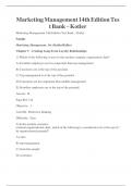
Inperfectcompetition,firmsandconsumersarep rice-takers
→thereisnomarketpower,nopossibilitytoaltertheprice
→afirmcansellasmuchoraslittleasitwantsattherulingmarketprice
→thedemandcurveforanindividualfirmisthereforeahorizontalline
Everyplayerinperfectcompetitionwill,asisnormal,chooseanoutputlevel
thatmaximisestheirindividualprofit.
→MC=MRandbecauseeachproductissoldatthemarketprice,
M
R=P=MC:pricethereforeequalsmarginalcostsinperfectcompetition
→foreveryindividualcompany,theoptimaloutputlevelqwillbesummed
andthisgivesustheaggregateoutputlevelQ
Themarketdemandcurvestillhasanegativeslope:
→iftheentiremarketoutputorpricechanges,theeffectisstillnoticeablein
thedemandcurve
(graphsareforo neindividualcompanyleftandforthee
ntiremarketright)
MONOPOLY
Ifthereisonlyonefirminthemarket,itsfirm'sdemandcurvewouldbeidenticaltothemarketdemand.
→itcouldsinglehandedlyinfluencethepriceasitcansinglehandedlychoosethesupply
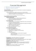
Asamonopolisthastheopportunitytochoosethequantity/priceashepleases,heisalso
facedwithaproductiondilemma:
−
→producingΔQ = Q2 Q1 moreunitsincreasesrevenuewithG
→b −
utdecreasedpricewithΔP = P 1 P 2 andthusrevenuewithL
Whatchoiceshouldthemonopolistmakeifhewantstomaximizeprofits?
Likeanyotherfirm,weneedtokeeptheoptimalityconditioninmind:MR=MC.
So,whatisMR?
× × −
→T R = q uantity price = Q (A B Q) = AQ B 2 Q −
⇒ dT R(Q)
M R = dQ = A 2BQ −
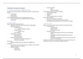
TheMR-curveofamonopolisthasthesameinterceptasitsdemandcurve,buttwicethe
slope.ThismeansthattheMR-curvewillalwaysliebeneaththedemandcurve.
Themaindifferencebetweenamonopolistandafirminperfectcompetitionisthat
theMRisn otequala nda lwayslessthantheactualmarketprice.
Followingtheoptimalityrule,MC=MR,themonopolistwillproductQM units
butwillsellthemataclearingpriceofP M
×
→thetotalrevenueQM P M isgreaterthanthetotalcostsAC(Q) QM ×
andthusthemonopolistattainsane conomicprofit.
Itisthereforeinteresting,foranyfirm,totryandachieveacertainlevelofmarketpower.
Inaperfectcompetition,economicprofitisbynomeanspossibleu nlessintheshortrun.
,PARTTWO
Inthiscourse,weadaptan eoclassicalapproachinwhichafirmissolelyenvisionedasaproduction
unit:thefirmtransformsinputsintooutputs:
→g oal:maximizeprofitsandhenceminimizetheproductioncosts
COSTRELATIONSHIPS
Afirmischaracterisedbyap roductionfunctionforasingleproductq.Thisfunctionspecifiesthequantity
qthatthefirmproducedfromusingkdifferentinputs:q = f (x1 , x2 , ..., xk )
Therelationshipbetweentheoutputchoice(productionfunction)andtheproductioncostsisexpressed
usingthec ostfunction:C (q) + F .Aswearelookingtomaximizeprofits,wewillsolve:
k
M inimize ∑ wi xi s.t. f (x1 , x2 , ..., xk ) = Q withQ=thechosenproductionlevel
i=1
solvingthislinearproblemfora
llquantitylevels,resultsintheoptimalcostfunction
wherecostsareminimized.
Thereare4categoriesofcosts:
1. Fixedcosts:agivenamountofexpenditurethatthefirmmustincure achp
eriodandthatis
unrelatedtohowmuchoutputthefirmproduces.
2. Averagecosts:thetotalcostsdividedbyoutput:
- Average F ixed Costs : F /Q
- Average V ariable Costs : C(Q)/Q
3. Marginalcosts:theadditiontototalcoststhatisincurredinincreasingoutputbyoneunit
→M arginal Costs : dC(Q)/dQ
4. Sunkcosts:coststhatarealsou nrelatedtotheoutput,butthatarespentbeforemeasuringthe
totalcosts(e.g.licences,researchexpenditures,...)andarealsou nrecoverableifthefirm
decidestoexitthemarket.
COSTVARIABLESANDOUTPUTDECISIONS
ProfitmaximizationoveranyperiodoftimerequiresthattheproducedwhereM C=MR.
Butitisimportanttonotethatthisisonlyapplicableifthecompanyproduces.
Acompanycanproduceinitsequilibriumbutthetotalrevenuecouldbesmallerthanthe
totalcosts.ThishappenswhentheequilibriumisundertheAVC-curve.
→inthiscase,thefirmwouldnotproduceandleavethemarket=s hut-downdecision
Inshort,outputdecisionsarebasedon:
1. MarginalCosts
→todecideh owmuchtoproduce:MC=MR
2. AverageCosts
→todecideifthefirmwillevenproduceinthelongrun
(lossesintheSRaretolerated,n otinthelongrun)
3. AverageVariableCosts
→todecideifthefirmwillevenproduceinthes hortrun
(price<ACcanbetolerated,price<AVCn otbecausetheneveryunitisaloss)
ECONOMIESOFSCALE
Thestateofaffairsinwhichaveragecostsfallasoutputincreases,meaningthatthecostperunitof
outputdeclinesasthescaleofoperationsrises.
⇒
→fallingAC-curve MC<AC
AC(Q)
WedefineS = M C(Q)
- ⇒
ifS>1 economiesofscale
- ⇒
ifS=1 m inimumefficientscale
- ⇒
ifS<1 diseconomiesofscale
,Weconcludethatthegreatertheextentofeconomiesofscale,thelargertheoutputatwhichtheaverage
costisminimized,thefewerfirmsthatcanoperateefficientlyinthemarket
⇒ largereconomiesofscaleforafewfirmswillresultinconcentratedmarkets
Now,whatcauseseconomiesofscale?
- underlyingtechnology
⇒
- greaterscaleofoperations specializationanddivisionoflabor
- economiesoninventory,repair,...
- capacityrelatedsolutions(e.g.volumeofcontainerthatincreasesexponentially)
ECONOMIESOFSCOPE
Thestateofaffairsinwhichitislesscostlytoproduceasetofgoodsinonefirmthanitistoproducethat
setintwoormorefirms.
WedefineS C =
−
C(q 1 , 0) + F 1 + C(0, q 2 ) + F [C(q 1 , q 2 ) + F ]
C(q 1 , q 2 ) + F
- ⇒
ifS>0 economiesofscope
- ⇒
ifS=0 criticalpoint,indifference
- ⇒
ifS<0 noeconomiesofscope
Theconceptofeconomiesofscopeisanimportantone,asitprovidesthecentraltechnologicalreason
fortheexistenceofmultiproductfirms.Therearetwocausesforeconomiesofscope:
1. Sharedinputs
→e.g.sharedR&D,equipmentthatcanbeusedformultipleproducts,...
2. Costcomplementarities
→producingonegoodreducesthecostofanother
MARKETSTRUCTURE
TheM arketStructureisdefinedastheamountandsizeoffirmswithinthatmarket+otherfactors.
Howtomeasurethemarketstructure?
- summarymeasures(e.g.numberoffirms,marketshareofeachfirm,...)
- concentrationcurve
- concentrationratios(e.g.C Rn )
- Herfindahl-HirschmanIndex(HII)
Summarymeasures
Mostofthetimesfairlyinaccurateasishardtolistallcompetitorswithinone
market.
ConcentrationCurve
Howlargearethelargestfirms?→cfr.steepnessofcurve
Howquicklydowereach100%?
…
ConcentrationRatios
e.g.C R4 =ratiothattellsyouhowmuchmarketsharethe4largestfirmsinamarkethavecombined.
Herfindahl-HirschmanIndex(HHI)
N
H HI = ∑ si2 =sumofs
quaredm
arketsharesofeachcompany.
i=1
, MARKETDEFINITION
Weunderstandthatitisimpossibletocalculatemetricsonthemarketstructure,ifwehavenoclear
definitionofthemarketwearestudying.Butdefiningamarketisnoeasythingtodo:
1. definebysubstitutabilityinp roduction
→standardapproach,basedonindustrycodes
→butlimitations
2. definebysubstitutabilityinc onsumption
→=d emandsubstitutability
→basedoncross-priceelasticity
Weshouldalsoaskourselves:w hatdrivespotentialmarketconcentration?
a. economiesofscale/economiesofscope
→largerfirmsbecomemoreefficient,concentrationrises
b. networkexternalities
→concentrated,eventhoughtherecouldbenoeconomiesofscale/scope
c. governmentandantitrustpolicy
→bylimitingentry,patentsystem,blockingofmergers,...
PARTTHREE
THECONCEPTOFDISCOUNTING
Boththecompetitionandmonopolymodelsaresomewhatvaguewithrespecttotime.
Asweknowmoneyhasatimevalue,themeaningofprofitorbreak-evenislessclear.
→weneedawaytoconverttomorrow'smoneyintotoday'smoney
⇒ wewillmakeuseofdiscountingandNetPresentValue
(Net)PresentValueisdirectlyrelevanttoprofitmaximization:
- foro ne-periodp roblems,wejustcontinuetousetheM R=MCoptimalityconstraint
- form ultiperiodp roblems,weneedtomakesurethatthepresentvalueoffutureincomestreams
mustatleastcoverthepresentvalueoftheexpensesinestablishingtheproject:P V-I>0
EFFICIENCYANDSURPLUS
Whyaremonopoliesoftenblocked?
→r eason:monopoliesareinefficient.
Efficiency:a marketoutcomeisefficientwhenitisimpossibletofindasmallchangeintheallocationof
capital,labor,goodsorservicesthatwouldimprovethewell-beingofindividualswithouthurtingothers.
→ananalysisofsurpluseswillgiveusanideaofwhyamonopolyisinefficientandthusunwanted
PERFECTCOMPETITION
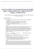
Efficiencyisbasicallyameasureofwell-being.
a. Consumersurplus:thedifferencebetweenthemaximumamountaconsumeris
⇒
willingtopay,andtheamountactuallypaid C S(aggregated)
b. Producersurplus:thedifferencebetweentheamountaproducerreceivesfroma
⇒
saleandtheamountthatthesalecosthim P S(aggregated)
Inthisdiagram(perfectcompetition),wecanseethatbothsurplusesaremaximized.
→thecompetitiveequilibriumise fficientandwelfareismaximized
SimonKuhn
LECTURE1:FOUNDATIONS
PARTONE
WHATISINDUSTRIALORGANISATION?
IndustrialOrganisationisabranchofeconomicsthatisconcernedwiththestudyofimperfect
competition.Wewilllookatwaysforacompanytoescapeperfectcompetition.
⇒ throughm arketpower:
- innovation
- advertisement
- productdifferentiation
- pricediscrimination
Inthiscourse,wewillusemanagerialeconomicstoanswerpracticalquestionsonthesetopics.
HOWWESTUDYINDUSTRIALORGANISATION
Wewillmakeuseof:
- fundamentaleconomicprinciples(e.g.rationalagents,optimality,...)
- gametheorybecauseofhighinterdependenceb etweenfirms
- abstractmodeling
THEPROBLEMOFTHEMANAGER
TheSmallBusinessAdministrationgivessomebasicguidelinesonhowtostructureabusinessplan:
- executivesummary→theuniquesellingpoint,whatdifferentiatesthebusinessfromothers
- companydescription→whichproductsandservices,productdifferentiation,...
- marketanalysis→economiesofscale,marketconcentration,sunkcosts,...
- serviceorproductline→ explainproductionprocesses,R&D,innovation,...
- marketingandsales→ describethemarketingstrategy,pricediscrimination,...
- financialplanandfunding
AlloftheseelementshavetodowithconceptsstudiedinManagerialEconomics.
→wewilllookattheeconomicsbehindtheseconceptswithin(im)perfectcompetition
inordertousethemformorepracticalapplications(e.g.abusinessplan)
MARKETDEMAND
InManagerialEconomics,wewillmainlyfocusonfirmprofit-maximizingbehaviorandaresultantmarket
outcomethatsuchbehaviorimplies.
MarketDemandCurved escribestherelationshipbetweenhowmuchmoney(aggregated)consumers
arewillingtopayperunitofthegoodandthequantity(aggregated)ofthegoodsconsumed.
→dependson:
- price
- income
- expectationsofpricemovement...
-⇒ Quantity = f (price, income, marketing, ...)
However,wewillexpressasimplifieddemandcurveintermsoftheprice:
1. Q = a bP −
- a=quantitydemandedwhenpriceisverysmall
- a/b=themaximumwillingnesstopay
⇒thisequationisusedwhenfirmshaveaf ixedquantitybutcaneasily
changetheprice(e.g.bakkery)=p rice-focused
−
2. P = A B Q ( inverse)
- A=themaximumwillingnesstopay
- A/B=quantitydemandedwhenpriceisverysmall
⇒thisequationisusedwhenfirmshaveav ariablequantity(inextremely
concentratedmarketse.g.oil,gold,...)=q uantity-focused
,Weneedtoaskourselveswhetheralinearmarketdemandcurveisevenrealistic?
- ithasaf unctionalform
→closertoanestimation,yetfairlyaccuratealocallevel
- itdoesnotakeintoaccountthet imefactor
a. shortrun:nopossibilitytochangeproductionfacilities
b. longrun:firmcanchangeitsproductionfacilitiestomeetdemand
→butmarketdemandcurvedoesnotmakethedistinction,thoughmarketschangeconstantly
- demandisafunctionofm anyaspects
→income(cfr.EngelLaw),Giffengoods,preferences,...
Yet,despiteitslimitations,wewillcontinuetousethesimple(inverse)lineardemand.
→weneedtoemphasisecompetition,notthedemandcurve
→easywaytofindtheequilibriuminanymarketsituation
FIRM'SDEMAND
TheF irm'sDemandg ivesacompanyanideahowmuchtheycansell,giventhepricetheyask:
a. ifthereisonlyo ⇒
nefirm thefirm'sdemandisequaltothemarketdemand
b. iftherearem ⇒
ultiplefirms thefirm'sdemanddependsonotherfirms:
⇒
QJ = f (P J , P K , income, marketing J , marketing K , ....)
Firmshaveanexplicit(e.g.throughquantitativemarketanalysis)orimplicit(e.g.gut-feeling)ofthe
⇒
marketdemand,andtheytrytoincreasetheirfirm'sdemand theyneedManagerialEconomics.
→agoodunderstandingofthefirm'sdemandisnecessary:indeed,wecannotstartproducingbefore
weknowwhatwecansell.
PRICEELASTICITYOFDEMAND
Elasticity:
⇒ε = ×
Δq
q Δq p Δq Δp
Δp = Δp q
with q = percentage change in q and p = percentage change in p
p
- if|ε| = 1 ⇒ifpricereduces/increases,thequantitywillreduce/increasebythesameamount
- if|ε| < 1 ⇒increasingpriceincreasesrevenues:d emandisinelastic
- if|ε| > 1 ⇒increasingpricereducesrevenues:d emandiselastic
Givenademandcurve,youwouldneedtofind:
Δq dq
- Δp = dp =thefirstderivativeoftheQ(p)function
- p/q =justfillin
Cross-elasticity:
⇒ε ×
Δq 1
q1 Δq 1 p2
1,2 = Δp2 = Δp2 q1
p2
- if|| ε1,2 || > 0 ⇒s ubstitutegoods
- if|| ε1,2 || < 0 ⇒c omplementgoods
,PERFECTCOMPETITION
Inperfectcompetition,firmsandconsumersarep rice-takers
→thereisnomarketpower,nopossibilitytoaltertheprice
→afirmcansellasmuchoraslittleasitwantsattherulingmarketprice
→thedemandcurveforanindividualfirmisthereforeahorizontalline
Everyplayerinperfectcompetitionwill,asisnormal,chooseanoutputlevel
thatmaximisestheirindividualprofit.
→MC=MRandbecauseeachproductissoldatthemarketprice,
M
R=P=MC:pricethereforeequalsmarginalcostsinperfectcompetition
→foreveryindividualcompany,theoptimaloutputlevelqwillbesummed
andthisgivesustheaggregateoutputlevelQ
Themarketdemandcurvestillhasanegativeslope:
→iftheentiremarketoutputorpricechanges,theeffectisstillnoticeablein
thedemandcurve
(graphsareforo neindividualcompanyleftandforthee
ntiremarketright)
MONOPOLY
Ifthereisonlyonefirminthemarket,itsfirm'sdemandcurvewouldbeidenticaltothemarketdemand.
→itcouldsinglehandedlyinfluencethepriceasitcansinglehandedlychoosethesupply
Asamonopolisthastheopportunitytochoosethequantity/priceashepleases,heisalso
facedwithaproductiondilemma:
−
→producingΔQ = Q2 Q1 moreunitsincreasesrevenuewithG
→b −
utdecreasedpricewithΔP = P 1 P 2 andthusrevenuewithL
Whatchoiceshouldthemonopolistmakeifhewantstomaximizeprofits?
Likeanyotherfirm,weneedtokeeptheoptimalityconditioninmind:MR=MC.
So,whatisMR?
× × −
→T R = q uantity price = Q (A B Q) = AQ B 2 Q −
⇒ dT R(Q)
M R = dQ = A 2BQ −
TheMR-curveofamonopolisthasthesameinterceptasitsdemandcurve,buttwicethe
slope.ThismeansthattheMR-curvewillalwaysliebeneaththedemandcurve.
Themaindifferencebetweenamonopolistandafirminperfectcompetitionisthat
theMRisn otequala nda lwayslessthantheactualmarketprice.
Followingtheoptimalityrule,MC=MR,themonopolistwillproductQM units
butwillsellthemataclearingpriceofP M
×
→thetotalrevenueQM P M isgreaterthanthetotalcostsAC(Q) QM ×
andthusthemonopolistattainsane conomicprofit.
Itisthereforeinteresting,foranyfirm,totryandachieveacertainlevelofmarketpower.
Inaperfectcompetition,economicprofitisbynomeanspossibleu nlessintheshortrun.
,PARTTWO
Inthiscourse,weadaptan eoclassicalapproachinwhichafirmissolelyenvisionedasaproduction
unit:thefirmtransformsinputsintooutputs:
→g oal:maximizeprofitsandhenceminimizetheproductioncosts
COSTRELATIONSHIPS
Afirmischaracterisedbyap roductionfunctionforasingleproductq.Thisfunctionspecifiesthequantity
qthatthefirmproducedfromusingkdifferentinputs:q = f (x1 , x2 , ..., xk )
Therelationshipbetweentheoutputchoice(productionfunction)andtheproductioncostsisexpressed
usingthec ostfunction:C (q) + F .Aswearelookingtomaximizeprofits,wewillsolve:
k
M inimize ∑ wi xi s.t. f (x1 , x2 , ..., xk ) = Q withQ=thechosenproductionlevel
i=1
solvingthislinearproblemfora
llquantitylevels,resultsintheoptimalcostfunction
wherecostsareminimized.
Thereare4categoriesofcosts:
1. Fixedcosts:agivenamountofexpenditurethatthefirmmustincure achp
eriodandthatis
unrelatedtohowmuchoutputthefirmproduces.
2. Averagecosts:thetotalcostsdividedbyoutput:
- Average F ixed Costs : F /Q
- Average V ariable Costs : C(Q)/Q
3. Marginalcosts:theadditiontototalcoststhatisincurredinincreasingoutputbyoneunit
→M arginal Costs : dC(Q)/dQ
4. Sunkcosts:coststhatarealsou nrelatedtotheoutput,butthatarespentbeforemeasuringthe
totalcosts(e.g.licences,researchexpenditures,...)andarealsou nrecoverableifthefirm
decidestoexitthemarket.
COSTVARIABLESANDOUTPUTDECISIONS
ProfitmaximizationoveranyperiodoftimerequiresthattheproducedwhereM C=MR.
Butitisimportanttonotethatthisisonlyapplicableifthecompanyproduces.
Acompanycanproduceinitsequilibriumbutthetotalrevenuecouldbesmallerthanthe
totalcosts.ThishappenswhentheequilibriumisundertheAVC-curve.
→inthiscase,thefirmwouldnotproduceandleavethemarket=s hut-downdecision
Inshort,outputdecisionsarebasedon:
1. MarginalCosts
→todecideh owmuchtoproduce:MC=MR
2. AverageCosts
→todecideifthefirmwillevenproduceinthelongrun
(lossesintheSRaretolerated,n otinthelongrun)
3. AverageVariableCosts
→todecideifthefirmwillevenproduceinthes hortrun
(price<ACcanbetolerated,price<AVCn otbecausetheneveryunitisaloss)
ECONOMIESOFSCALE
Thestateofaffairsinwhichaveragecostsfallasoutputincreases,meaningthatthecostperunitof
outputdeclinesasthescaleofoperationsrises.
⇒
→fallingAC-curve MC<AC
AC(Q)
WedefineS = M C(Q)
- ⇒
ifS>1 economiesofscale
- ⇒
ifS=1 m inimumefficientscale
- ⇒
ifS<1 diseconomiesofscale
,Weconcludethatthegreatertheextentofeconomiesofscale,thelargertheoutputatwhichtheaverage
costisminimized,thefewerfirmsthatcanoperateefficientlyinthemarket
⇒ largereconomiesofscaleforafewfirmswillresultinconcentratedmarkets
Now,whatcauseseconomiesofscale?
- underlyingtechnology
⇒
- greaterscaleofoperations specializationanddivisionoflabor
- economiesoninventory,repair,...
- capacityrelatedsolutions(e.g.volumeofcontainerthatincreasesexponentially)
ECONOMIESOFSCOPE
Thestateofaffairsinwhichitislesscostlytoproduceasetofgoodsinonefirmthanitistoproducethat
setintwoormorefirms.
WedefineS C =
−
C(q 1 , 0) + F 1 + C(0, q 2 ) + F [C(q 1 , q 2 ) + F ]
C(q 1 , q 2 ) + F
- ⇒
ifS>0 economiesofscope
- ⇒
ifS=0 criticalpoint,indifference
- ⇒
ifS<0 noeconomiesofscope
Theconceptofeconomiesofscopeisanimportantone,asitprovidesthecentraltechnologicalreason
fortheexistenceofmultiproductfirms.Therearetwocausesforeconomiesofscope:
1. Sharedinputs
→e.g.sharedR&D,equipmentthatcanbeusedformultipleproducts,...
2. Costcomplementarities
→producingonegoodreducesthecostofanother
MARKETSTRUCTURE
TheM arketStructureisdefinedastheamountandsizeoffirmswithinthatmarket+otherfactors.
Howtomeasurethemarketstructure?
- summarymeasures(e.g.numberoffirms,marketshareofeachfirm,...)
- concentrationcurve
- concentrationratios(e.g.C Rn )
- Herfindahl-HirschmanIndex(HII)
Summarymeasures
Mostofthetimesfairlyinaccurateasishardtolistallcompetitorswithinone
market.
ConcentrationCurve
Howlargearethelargestfirms?→cfr.steepnessofcurve
Howquicklydowereach100%?
…
ConcentrationRatios
e.g.C R4 =ratiothattellsyouhowmuchmarketsharethe4largestfirmsinamarkethavecombined.
Herfindahl-HirschmanIndex(HHI)
N
H HI = ∑ si2 =sumofs
quaredm
arketsharesofeachcompany.
i=1
, MARKETDEFINITION
Weunderstandthatitisimpossibletocalculatemetricsonthemarketstructure,ifwehavenoclear
definitionofthemarketwearestudying.Butdefiningamarketisnoeasythingtodo:
1. definebysubstitutabilityinp roduction
→standardapproach,basedonindustrycodes
→butlimitations
2. definebysubstitutabilityinc onsumption
→=d emandsubstitutability
→basedoncross-priceelasticity
Weshouldalsoaskourselves:w hatdrivespotentialmarketconcentration?
a. economiesofscale/economiesofscope
→largerfirmsbecomemoreefficient,concentrationrises
b. networkexternalities
→concentrated,eventhoughtherecouldbenoeconomiesofscale/scope
c. governmentandantitrustpolicy
→bylimitingentry,patentsystem,blockingofmergers,...
PARTTHREE
THECONCEPTOFDISCOUNTING
Boththecompetitionandmonopolymodelsaresomewhatvaguewithrespecttotime.
Asweknowmoneyhasatimevalue,themeaningofprofitorbreak-evenislessclear.
→weneedawaytoconverttomorrow'smoneyintotoday'smoney
⇒ wewillmakeuseofdiscountingandNetPresentValue
(Net)PresentValueisdirectlyrelevanttoprofitmaximization:
- foro ne-periodp roblems,wejustcontinuetousetheM R=MCoptimalityconstraint
- form ultiperiodp roblems,weneedtomakesurethatthepresentvalueoffutureincomestreams
mustatleastcoverthepresentvalueoftheexpensesinestablishingtheproject:P V-I>0
EFFICIENCYANDSURPLUS
Whyaremonopoliesoftenblocked?
→r eason:monopoliesareinefficient.
Efficiency:a marketoutcomeisefficientwhenitisimpossibletofindasmallchangeintheallocationof
capital,labor,goodsorservicesthatwouldimprovethewell-beingofindividualswithouthurtingothers.
→ananalysisofsurpluseswillgiveusanideaofwhyamonopolyisinefficientandthusunwanted
PERFECTCOMPETITION
Efficiencyisbasicallyameasureofwell-being.
a. Consumersurplus:thedifferencebetweenthemaximumamountaconsumeris
⇒
willingtopay,andtheamountactuallypaid C S(aggregated)
b. Producersurplus:thedifferencebetweentheamountaproducerreceivesfroma
⇒
saleandtheamountthatthesalecosthim P S(aggregated)
Inthisdiagram(perfectcompetition),wecanseethatbothsurplusesaremaximized.
→thecompetitiveequilibriumise fficientandwelfareismaximized