Summary Statistics 3
exam 2021
Unit 1: contingency tables, odds
ratios, stratification, confounding
and interaction
The 2X2 contingency table for association
X=0/ control X=1/ treated
Y=0/ no recovery 13 (A) 7 (B) 20 (A+B)
Y=1/ recovery 12 (C) 18 (D) 30 (C+D)
25 (A+C) 25 (B+D) N=50
The null hypothesis is that there is no effect of therapy on the probability of recovery. This is the same as:
P (recovered | therapy) = P (recovered | control)
the probability of recovery (i.e. the marginal probability, which is the probability of a single event
occurring independent of other events) is 30/50, which is 0.6, which is 60%. we’d expect that in both
groups 60% recovers 60% x 25 (amount of people in each group)= 15, we expect 15 people to recover
and 10 to not recover.
an alternative null hypothesis would be that there is no association between therapy and recovery, which
is P (recovery AND treated) = P (recovery) * P (treated). Given that 30/50 people recover, and 25 out of
50 are treated, the probability of a patient being treated and recovering is; (30/50) * (25/50)= 30%. The
total sample size is 50 15 people in the cell recovery AND treated, by the same logic we expect 15
people in the recovery AND control cell, and 10 patients in each of the other 2 cells.
What we have used here is the product rule for independent events. If there’s no association between X
and Y this implies that therapy and recovery are statistically independent. If they are, the probability of
both occurring simultaneously is the product of the unconditional probabilities.
The table above shows the observed frequencies, the values we have calculated are the expected
frequencies under the H0. We calculate the expected frequency as follows: row total * column total/
grand total:
X0 X1
Y0 20*25/50= 10 20*25/50=10 20
Y1 30*25/50=15 30*25/50=15 30
25 25 50
,Test of association in contingency table
2 2 2
(O −E rc)
χ =∑ ∑ rc
2
,df =1
r=1 c=1 Erc
For each cell r, c (r=row, c=column) we take the difference between the observed and expected
frequency
We raise this difference to the power of 2 and then divide by Erc
We sum these terms over the 2 columns and rows
This test is an approximation and requires that all E’s are at least 5 or more.
X0 X1
Y0 (13-10)2/10= 0.9 (7-10)2/10= 0.9 1.8
2 2
Y1 (12-15) /15=0.6 (18-15) /15= 0.6 1.2
1.5 1.5 3= χ 2
Under the H0 this test statistic has a Chi-square distribution with df=1, since the derivations O-E are raised
to the power of 2, a violation of the H0 leads to large Chi-square values the critical area is on the right
of the distribution. If we now look at the Chi-square distributions, the critical value is 3.84, values larger
than this lead to rejection of the H0.
We cannot reject our H0 but we cannot accept it either the power to detect a true statement effect
may be too small with N=50. The 95% confidence interval runs from -0.02 to +0.5 the true difference
can be 0 as H0 claims, or anything up to 50%.
Measures of association for 2X2 contingency
table
The effect of treatment on recovery probability can be expressed in 3 different ways:
1. The difference in recovery probability
2. The correlation between treatment and recovery
3. The odds ratio
Applying the formula for Pearson’s correlation r to 0/1 variables (dichotomous) and rewriting the formula
gives us what is known as the phi-coefficient (φ):
( A x D ) −( B x C)
φ=
√( A+ B )( A+C ) ( B+ D )(C+ D)
The A, B, C and D are the same as in the first table. Note that A (00, not treated and not recovered) and D
(11, treated and recovered) contribute to a positive correlation between treatment and recovery. B and C
contribute to a negative correlation.
The Odds Ratio (OR) is defined as follows:
The odds are defined as P (Y=1)/ P (Y=0), i.e. the probability of success divided by the probability
of failure
The Odds Ratio is the ratio of the odds of the group (X=1) to the odds of the group (X=0)
, D/B A∗D
The OR: =
C/ A B∗C
The OR is equal to the number of concordant pairs (contribute to positive correlation) divided by the
number of discordant pairs (contribute to negative correlations)
situation Phi- coefficient Odds ratio Association?
A*D> B*C >0 >1 Positive association
A*D=B*C =0 =1 No association
A*D<B*C <0 <1 Negative association
The OR in our example is thus; (13*18)/(7*12)=2.79, this value is larger than 1 and thus there is a positive
association. The phi coefficient is 0.25.
But what does this mean when we have binary variables? We need to think about the coding: the value of
X=1 tends to go with the value of Y=1.
The 2X2X2 contingency
table: stratification
In analysing the relationship between predictor X and
outcome Y, we might want to adjust for a 3rd variable C.
we need to distinguish between different causal models
and roles for C.
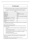
The confounding model
X and C can both affect Y, and X and C are correlated
with each other (they are confounded) but neither
of the 2 have an effect on the other. In this case we
suppose that C=1 is for the mild cases of depression
and C=0 for the severe cases.
We need to adjust the effect of X on Y for C,
because otherwise the effect of X will be
biased.
The mediation model
X affects C which in turn affects Y, X can also still affect Y directly (this concept is not really discussed in
the course). In this case we suppose C=compliance
The difference between mediation and confounding is that we always want to correct for confounding,
whereas this is not always the case with mediation where this might be of scientific interest.
, The moderation (interaction) model
The effect of X on Y depends on the value of C. C in this case could be the level of depression at pretest
where Y is the level of depression at posttest. We need to test the simple effect of X per value of C.
Now what do we do with a confounder or moderator? We break down the contingency table, i.e. we
stratify it for all levels of C, and perform logistic regression analyses.
Working with logarithms
For reasons to be seen in the following unit, we often take the natural logarithm of the odds ratio.
Ln (a) + ln(b)= Ln (a*b)
Ln (a)- ln (b)= ln (a/b)
Goes if a and b >0
Ln (ab)= b * ln (a)
Ln (1/a)= -ln (a)
Goes if a>0
Special logarithms:
Ln (odds)= ln (P) – ln (1-P)
Ln (OR)= ln (oddsx=1) – ln (oddsx=0)
Ln (1)= 0, ln (e)=1 (e≈2.72)
Now why would we use these (they look confusing AF)? probability is bounded between 0 and 1 but
log odds are not they go from minus infinity to plus infinity and this allows us to analyse the data as if we
were working with quantitative variables, i.e. it allows for easier interpretation.
If we work with log odds transformations and X= 0/1 the slope of the logistic function is equal to the ln
(OR).
Working with exponentials
Exp(a) * exp(b)= exp (a+b)
Exp (a)/ exp (b)= exp (a-b)
[exp(a)]b= exp (a*b)
1/ exp (a)= exp(-a)
An exponential is the inverse of a logarithm
(whatever that means?!).
Special powers of e:
Exp(ln(a))= ln (exp(a))= a, if a>0
Exp(0)=1
Exp(1)=e ≈2.72
The logarithms and exponentials together allow us to switch from one scale to another.
exam 2021
Unit 1: contingency tables, odds
ratios, stratification, confounding
and interaction
The 2X2 contingency table for association
X=0/ control X=1/ treated
Y=0/ no recovery 13 (A) 7 (B) 20 (A+B)
Y=1/ recovery 12 (C) 18 (D) 30 (C+D)
25 (A+C) 25 (B+D) N=50
The null hypothesis is that there is no effect of therapy on the probability of recovery. This is the same as:
P (recovered | therapy) = P (recovered | control)
the probability of recovery (i.e. the marginal probability, which is the probability of a single event
occurring independent of other events) is 30/50, which is 0.6, which is 60%. we’d expect that in both
groups 60% recovers 60% x 25 (amount of people in each group)= 15, we expect 15 people to recover
and 10 to not recover.
an alternative null hypothesis would be that there is no association between therapy and recovery, which
is P (recovery AND treated) = P (recovery) * P (treated). Given that 30/50 people recover, and 25 out of
50 are treated, the probability of a patient being treated and recovering is; (30/50) * (25/50)= 30%. The
total sample size is 50 15 people in the cell recovery AND treated, by the same logic we expect 15
people in the recovery AND control cell, and 10 patients in each of the other 2 cells.
What we have used here is the product rule for independent events. If there’s no association between X
and Y this implies that therapy and recovery are statistically independent. If they are, the probability of
both occurring simultaneously is the product of the unconditional probabilities.
The table above shows the observed frequencies, the values we have calculated are the expected
frequencies under the H0. We calculate the expected frequency as follows: row total * column total/
grand total:
X0 X1
Y0 20*25/50= 10 20*25/50=10 20
Y1 30*25/50=15 30*25/50=15 30
25 25 50
,Test of association in contingency table
2 2 2
(O −E rc)
χ =∑ ∑ rc
2
,df =1
r=1 c=1 Erc
For each cell r, c (r=row, c=column) we take the difference between the observed and expected
frequency
We raise this difference to the power of 2 and then divide by Erc
We sum these terms over the 2 columns and rows
This test is an approximation and requires that all E’s are at least 5 or more.
X0 X1
Y0 (13-10)2/10= 0.9 (7-10)2/10= 0.9 1.8
2 2
Y1 (12-15) /15=0.6 (18-15) /15= 0.6 1.2
1.5 1.5 3= χ 2
Under the H0 this test statistic has a Chi-square distribution with df=1, since the derivations O-E are raised
to the power of 2, a violation of the H0 leads to large Chi-square values the critical area is on the right
of the distribution. If we now look at the Chi-square distributions, the critical value is 3.84, values larger
than this lead to rejection of the H0.
We cannot reject our H0 but we cannot accept it either the power to detect a true statement effect
may be too small with N=50. The 95% confidence interval runs from -0.02 to +0.5 the true difference
can be 0 as H0 claims, or anything up to 50%.
Measures of association for 2X2 contingency
table
The effect of treatment on recovery probability can be expressed in 3 different ways:
1. The difference in recovery probability
2. The correlation between treatment and recovery
3. The odds ratio
Applying the formula for Pearson’s correlation r to 0/1 variables (dichotomous) and rewriting the formula
gives us what is known as the phi-coefficient (φ):
( A x D ) −( B x C)
φ=
√( A+ B )( A+C ) ( B+ D )(C+ D)
The A, B, C and D are the same as in the first table. Note that A (00, not treated and not recovered) and D
(11, treated and recovered) contribute to a positive correlation between treatment and recovery. B and C
contribute to a negative correlation.
The Odds Ratio (OR) is defined as follows:
The odds are defined as P (Y=1)/ P (Y=0), i.e. the probability of success divided by the probability
of failure
The Odds Ratio is the ratio of the odds of the group (X=1) to the odds of the group (X=0)
, D/B A∗D
The OR: =
C/ A B∗C
The OR is equal to the number of concordant pairs (contribute to positive correlation) divided by the
number of discordant pairs (contribute to negative correlations)
situation Phi- coefficient Odds ratio Association?
A*D> B*C >0 >1 Positive association
A*D=B*C =0 =1 No association
A*D<B*C <0 <1 Negative association
The OR in our example is thus; (13*18)/(7*12)=2.79, this value is larger than 1 and thus there is a positive
association. The phi coefficient is 0.25.
But what does this mean when we have binary variables? We need to think about the coding: the value of
X=1 tends to go with the value of Y=1.
The 2X2X2 contingency
table: stratification
In analysing the relationship between predictor X and
outcome Y, we might want to adjust for a 3rd variable C.
we need to distinguish between different causal models
and roles for C.
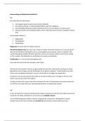
The confounding model
X and C can both affect Y, and X and C are correlated
with each other (they are confounded) but neither
of the 2 have an effect on the other. In this case we
suppose that C=1 is for the mild cases of depression
and C=0 for the severe cases.
We need to adjust the effect of X on Y for C,
because otherwise the effect of X will be
biased.
The mediation model
X affects C which in turn affects Y, X can also still affect Y directly (this concept is not really discussed in
the course). In this case we suppose C=compliance
The difference between mediation and confounding is that we always want to correct for confounding,
whereas this is not always the case with mediation where this might be of scientific interest.
, The moderation (interaction) model
The effect of X on Y depends on the value of C. C in this case could be the level of depression at pretest
where Y is the level of depression at posttest. We need to test the simple effect of X per value of C.
Now what do we do with a confounder or moderator? We break down the contingency table, i.e. we
stratify it for all levels of C, and perform logistic regression analyses.
Working with logarithms
For reasons to be seen in the following unit, we often take the natural logarithm of the odds ratio.
Ln (a) + ln(b)= Ln (a*b)
Ln (a)- ln (b)= ln (a/b)
Goes if a and b >0
Ln (ab)= b * ln (a)
Ln (1/a)= -ln (a)
Goes if a>0
Special logarithms:
Ln (odds)= ln (P) – ln (1-P)
Ln (OR)= ln (oddsx=1) – ln (oddsx=0)
Ln (1)= 0, ln (e)=1 (e≈2.72)
Now why would we use these (they look confusing AF)? probability is bounded between 0 and 1 but
log odds are not they go from minus infinity to plus infinity and this allows us to analyse the data as if we
were working with quantitative variables, i.e. it allows for easier interpretation.
If we work with log odds transformations and X= 0/1 the slope of the logistic function is equal to the ln
(OR).
Working with exponentials
Exp(a) * exp(b)= exp (a+b)
Exp (a)/ exp (b)= exp (a-b)
[exp(a)]b= exp (a*b)
1/ exp (a)= exp(-a)
An exponential is the inverse of a logarithm
(whatever that means?!).
Special powers of e:
Exp(ln(a))= ln (exp(a))= a, if a>0
Exp(0)=1
Exp(1)=e ≈2.72
The logarithms and exponentials together allow us to switch from one scale to another.