end
end
% p =
%
% 0 0.0199 0.9801
% 0.0023 0.0068 0.9909
% 0.0033 0.0047 0.9921
% 0.0023 0.0020 0.9957
% 0.0023 0.0005 0.9973
% 0.0036 0.0000 0.9964
% 0.0066 0 0.9934
% 0 0 1.0000
15. (a)
α1 δ(τ ) ρ = 70Hz
S(τ, ρ) = α2 δ(τ − 0.022µsec) ρ = 49.5Hz
0 else
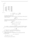
The antenna setup is shown in Fig. 15
From the figure, the distance travelled by the LOS ray is d and the distance travelled by the first
multipath component is sµ 
d 2
2 + 64
2
Given this setup, we can plot the arrival of the LOS ray and the multipath ray that bounces off
the ground on a time axis as shown in Fig. 15
So we have sµ 
d 2
2 + 82 − d = 0.022 × 10⁻⁶ 3 × 10⁸
2
µ 2 
d
⇒4 + 82 = 6.62 + d2 + 2d(6.6)
4
⇒ d = 16.1m
fD = v cos(θ)/λ. v = fD λ/ cos(θ). For the LOS ray, θ = 0 and for the multipath component,
θ = 45o . We can use either of these rays and the corresponding fD value to get v = 23.33m/s.
(b)
4ht hr
dc =
λ
dc = 768 m. Since d ¿ dc , power fall-off is proportional to d−2 .
(c) Tm = 0.022µs, B −1 = 0.33µs. Since Tm ¿ B −1 , we have flat fading.
16. (a) Outdoor, since delay spread ≈ 10 µsec.
Consider that 10 µsec ⇒ d = ct = 3km difference between length of first and last path
(b) Scattering function
S(τ, ρ) = F∆t [Ac (τ, ∆t)]
1
¡
1
¢
= W rect W ρ for 0 ≤ τ ≤ 10µsec
The Scattering function is plotted in Fig. 16
,8m 8m
d meters
Figure 4: Antenna Setting
0.022 us
0 t0 t1 t
t0 = (d/3e8)
t1 = 2 sqrt[(d/2)^2+8^2]/3e8
Figure 5: Time Axis for Ray Arrival
R
∞
τ Ac (τ )dτ
0
(c) Avg Delay Spread = R
∞ = 5µsec
Ac (τ )dτ
v 0
u∞
u R (τ −µT m )2 Ac (τ )dτ
u
RMS Delay Spread = t 0 ∞ R = 2.89µsec
Ac (τ )dτ
0
W
Doppler Spread = 2 = 50 Hz
1
(d) βu > Coherence BW ⇒ Freq. Selective Fading ≈ Tm = 105 ⇒ βu > = 105 kHz
Can also use µT m or σT m instead of Tm
(e) Rayleigh fading, since receiver power is evenly distributed relative to delay; no dominant LOS
path
2
eρ √
−1 W
(f) tR = ρFD 2π
with ρ = 1, fD = 2 → tr = .0137 sec
(g) Notice that the fade duration never becomes more than twice the average. So, if we choose our
data rate such that a single symbol spans the average fade duration, in the worst case two symbols
will span the fade duration. So our code can correct for the lost symbols and we will have error-free
transmission. So t1R = 72.94 symbols/sec
17. (a) Tm ≈ .1msec = 100µsec
Bd ≈ .1Hz
Answers based on µTm or σTm are fine too. Notice, that based on the choice of either Tm , µTm or
σTm , the remaining answers will be different too.
(b) Bc ≈ T1m = 10kHz
∆f > 10kHz for u1 ⊥ u2
(c) (∆t)c = 10s
(d) 3kHz < Bc ⇒ Flat
30kHz > Bc ⇒ Freq. Selective
, S(tau,rho)
-W/2 W/2 rho
10 us
tau
Figure 6: Scattering Function
end
% p =
%
% 0 0.0199 0.9801
% 0.0023 0.0068 0.9909
% 0.0033 0.0047 0.9921
% 0.0023 0.0020 0.9957
% 0.0023 0.0005 0.9973
% 0.0036 0.0000 0.9964
% 0.0066 0 0.9934
% 0 0 1.0000
15. (a)
α1 δ(τ ) ρ = 70Hz
S(τ, ρ) = α2 δ(τ − 0.022µsec) ρ = 49.5Hz
0 else
The antenna setup is shown in Fig. 15
From the figure, the distance travelled by the LOS ray is d and the distance travelled by the first
multipath component is sµ 
d 2
2 + 64
2
Given this setup, we can plot the arrival of the LOS ray and the multipath ray that bounces off
the ground on a time axis as shown in Fig. 15
So we have sµ 
d 2
2 + 82 − d = 0.022 × 10⁻⁶ 3 × 10⁸
2
µ 2 
d
⇒4 + 82 = 6.62 + d2 + 2d(6.6)
4
⇒ d = 16.1m
fD = v cos(θ)/λ. v = fD λ/ cos(θ). For the LOS ray, θ = 0 and for the multipath component,
θ = 45o . We can use either of these rays and the corresponding fD value to get v = 23.33m/s.
(b)
4ht hr
dc =
λ
dc = 768 m. Since d ¿ dc , power fall-off is proportional to d−2 .
(c) Tm = 0.022µs, B −1 = 0.33µs. Since Tm ¿ B −1 , we have flat fading.
16. (a) Outdoor, since delay spread ≈ 10 µsec.
Consider that 10 µsec ⇒ d = ct = 3km difference between length of first and last path
(b) Scattering function
S(τ, ρ) = F∆t [Ac (τ, ∆t)]
1
¡
1
¢
= W rect W ρ for 0 ≤ τ ≤ 10µsec
The Scattering function is plotted in Fig. 16
,8m 8m
d meters
Figure 4: Antenna Setting
0.022 us
0 t0 t1 t
t0 = (d/3e8)
t1 = 2 sqrt[(d/2)^2+8^2]/3e8
Figure 5: Time Axis for Ray Arrival
R
∞
τ Ac (τ )dτ
0
(c) Avg Delay Spread = R
∞ = 5µsec
Ac (τ )dτ
v 0
u∞
u R (τ −µT m )2 Ac (τ )dτ
u
RMS Delay Spread = t 0 ∞ R = 2.89µsec
Ac (τ )dτ
0
W
Doppler Spread = 2 = 50 Hz
1
(d) βu > Coherence BW ⇒ Freq. Selective Fading ≈ Tm = 105 ⇒ βu > = 105 kHz
Can also use µT m or σT m instead of Tm
(e) Rayleigh fading, since receiver power is evenly distributed relative to delay; no dominant LOS
path
2
eρ √
−1 W
(f) tR = ρFD 2π
with ρ = 1, fD = 2 → tr = .0137 sec
(g) Notice that the fade duration never becomes more than twice the average. So, if we choose our
data rate such that a single symbol spans the average fade duration, in the worst case two symbols
will span the fade duration. So our code can correct for the lost symbols and we will have error-free
transmission. So t1R = 72.94 symbols/sec
17. (a) Tm ≈ .1msec = 100µsec
Bd ≈ .1Hz
Answers based on µTm or σTm are fine too. Notice, that based on the choice of either Tm , µTm or
σTm , the remaining answers will be different too.
(b) Bc ≈ T1m = 10kHz
∆f > 10kHz for u1 ⊥ u2
(c) (∆t)c = 10s
(d) 3kHz < Bc ⇒ Flat
30kHz > Bc ⇒ Freq. Selective
, S(tau,rho)
-W/2 W/2 rho
10 us
tau
Figure 6: Scattering Function