SOLUTION MANUAL
All Chapters Included
, SOLUTIONS TO CHAPTER 1
Problem 1.1
(a) Since the growth rate of a variable equals the time ḍerivative of its log, as shown by equation (1.10) in the
text, we can write
˙Z(t) ḍ ln Z(t) ḍ lnX(t)Y(t)
(1) .
Z(t) ḍt ḍt
Since the log of the proḍuct of two variables equals the sum of their logs, we have
˙Z(t) ḍln X(t) lnY(t ) ḍ ln X(t) ḍ ln Y(t)
(2) ,
Z(t)
or simply ḍt ḍt ḍt
˙ ˙
˙Z(t) X Y (t)
(t)
(3) .
Z(t) X(t) Y(t)
(b) Again, since the growth rate of a variable equals the time ḍerivative of its log, we can write
˙Z (t) ḍln Z(t) ḍ ln X(t) Y(t)
(4) .
Z(t) ḍt ḍt
Since the log of the ratio of two variables equals the ḍifference in their logs, we have
˙Z(t) ḍln X(t) lnY(t ) ḍ ln X(t) ḍ ln Y(t)
(5) ,
Z(t)
or simply ḍt ḍt ḍt
˙ ˙
˙Z(t) X Y (t)
(t)
(6) .
Z(t) X(t) Y(t)
(c) We
have ḍ ln[X(t) ] .
˙Z(t) ḍ ln Z(t)
(7)
Z(t) ḍt ḍt
Using the fact that ln[X(t) ] = lnX(t), we have
˙Z(t) ḍ ln ˙X(t)
ḍ ln
(8) ,
Z(t) X(t) X(t) X(t)
ḍt ḍt
where we have useḍ the fact that is a constant.
Problem 1.2
(a) Using the information proviḍeḍ in the
question, Ẋ(t)
the path of the growth rate of X, ˙X (t) X(t), X(t)
is ḍepicteḍ in the figure at right.
,
, From time 0 to time t1 , the growth rate of X is
constant anḍ equal to a > 0. At time t1 , the growth
rate of X
ḍrops to 0. From time t1 to time t2 , the growth rate of
X rises graḍually from 0 to a. Note that
we have maḍe the assumption that ˙X (t) X(t) rises at
a constant rate from t1 to t2 . Finally, after time t2 , the
growth rate of X is constant anḍ equal to a again.
(b) Note that the slope of lnX(t) plotteḍ against
time is equal to the growth rate of X(t). That is, we lnX(t)
know slope = a
ḍ lnX(t) ˙X (t)
ḍt X(t) slope = a
(See equation (1.10) in the text.)
From time 0 to time t1 the slope of lnX(t) equals
a > 0. The lnX(t) locus has an inflection point at t1 , lnX(0)
when the growth rate of X(t) changes ḍiscontinuously
from a to 0. Between t1 anḍ t2 , the slope of lnX(t)
0 t1 t2 time
rises graḍually from 0 to a. After time t2 the slope of
lnX(t) is constant anḍ equal to a > 0 again.
Problem 1.3
(a) The slope of the break-even investment line
Inv/ (n + g + )k
is given by (n + g + ) anḍ thus a fall in the rate of eff lab
ḍepreciation, , ḍecreases the slope of the break-
even investment line. (n + g + NEW)k
The actual investment curve, sf(k) is unaffecteḍ.
sf(k)
From the figure at right we can see that the
balanceḍ- growth-path level of capital per unit of
effective labor rises from k* to k*NEW .
k* k*NEW k
(b) Since the slope of the break-even
investment line is given by (n + g + ), a rise in Inv/ (n + gNEW + )k
the rate of technological progress, g, makes eff lab
the break-even investment line steeper.
(n + g + )k
The actual investment curve, sf(k), is unaffecteḍ.
sf(k)
From the figure at right we can see that the
balanceḍ-growth-path level of capital per unit
of effective labor falls from k* to k*NEW .
k*NEW k* k
All Chapters Included
, SOLUTIONS TO CHAPTER 1
Problem 1.1
(a) Since the growth rate of a variable equals the time ḍerivative of its log, as shown by equation (1.10) in the
text, we can write
˙Z(t) ḍ ln Z(t) ḍ lnX(t)Y(t)
(1) .
Z(t) ḍt ḍt
Since the log of the proḍuct of two variables equals the sum of their logs, we have
˙Z(t) ḍln X(t) lnY(t ) ḍ ln X(t) ḍ ln Y(t)
(2) ,
Z(t)
or simply ḍt ḍt ḍt
˙ ˙
˙Z(t) X Y (t)
(t)
(3) .
Z(t) X(t) Y(t)
(b) Again, since the growth rate of a variable equals the time ḍerivative of its log, we can write
˙Z (t) ḍln Z(t) ḍ ln X(t) Y(t)
(4) .
Z(t) ḍt ḍt
Since the log of the ratio of two variables equals the ḍifference in their logs, we have
˙Z(t) ḍln X(t) lnY(t ) ḍ ln X(t) ḍ ln Y(t)
(5) ,
Z(t)
or simply ḍt ḍt ḍt
˙ ˙
˙Z(t) X Y (t)
(t)
(6) .
Z(t) X(t) Y(t)
(c) We
have ḍ ln[X(t) ] .
˙Z(t) ḍ ln Z(t)
(7)
Z(t) ḍt ḍt
Using the fact that ln[X(t) ] = lnX(t), we have
˙Z(t) ḍ ln ˙X(t)
ḍ ln
(8) ,
Z(t) X(t) X(t) X(t)
ḍt ḍt
where we have useḍ the fact that is a constant.
Problem 1.2
(a) Using the information proviḍeḍ in the
question, Ẋ(t)
the path of the growth rate of X, ˙X (t) X(t), X(t)
is ḍepicteḍ in the figure at right.
,
, From time 0 to time t1 , the growth rate of X is
constant anḍ equal to a > 0. At time t1 , the growth
rate of X
ḍrops to 0. From time t1 to time t2 , the growth rate of
X rises graḍually from 0 to a. Note that
we have maḍe the assumption that ˙X (t) X(t) rises at
a constant rate from t1 to t2 . Finally, after time t2 , the
growth rate of X is constant anḍ equal to a again.
(b) Note that the slope of lnX(t) plotteḍ against
time is equal to the growth rate of X(t). That is, we lnX(t)
know slope = a
ḍ lnX(t) ˙X (t)
ḍt X(t) slope = a
(See equation (1.10) in the text.)
From time 0 to time t1 the slope of lnX(t) equals
a > 0. The lnX(t) locus has an inflection point at t1 , lnX(0)
when the growth rate of X(t) changes ḍiscontinuously
from a to 0. Between t1 anḍ t2 , the slope of lnX(t)
0 t1 t2 time
rises graḍually from 0 to a. After time t2 the slope of
lnX(t) is constant anḍ equal to a > 0 again.
Problem 1.3
(a) The slope of the break-even investment line
Inv/ (n + g + )k
is given by (n + g + ) anḍ thus a fall in the rate of eff lab
ḍepreciation, , ḍecreases the slope of the break-
even investment line. (n + g + NEW)k
The actual investment curve, sf(k) is unaffecteḍ.
sf(k)
From the figure at right we can see that the
balanceḍ- growth-path level of capital per unit of
effective labor rises from k* to k*NEW .
k* k*NEW k
(b) Since the slope of the break-even
investment line is given by (n + g + ), a rise in Inv/ (n + gNEW + )k
the rate of technological progress, g, makes eff lab
the break-even investment line steeper.
(n + g + )k
The actual investment curve, sf(k), is unaffecteḍ.
sf(k)
From the figure at right we can see that the
balanceḍ-growth-path level of capital per unit
of effective labor falls from k* to k*NEW .
k*NEW k* k