INSTRUCTOR’S SOLUTIONS MANUAL
DIFFERENTIAL EQUATIONS AND BOUNDARY VALUE PROBLEMS
6TH EDITION
CHAPTER NO. 01: FIRST-ORDER DIFFERENTIAL EQUATIONS
SECTION 1.1
DIFFERENTIAL EQUATIONS AND MATHEMATICAL MODELS
The main purpose of Section 1.1 is simply to introduce the basic notation and terminology of dif-
ferential equations, and to show the student what is meant by a solution of a differential
equation. Also, the use of differential equations in the mathematical modeling of real-world
phenomena is outlined.
Problems 1-12 are routine verifications by direct substitution of the suggested solutions into the
given differential equations. We include here just some typical examples of such verifications.
3. If y1 cos 2 x and y2 sin 2 x , then y1 2sin 2 x y2 2 cos 2 x , so
y1 4 cos 2 x 4 y1 and y2 4sin 2 x 4 y2 . Thus y1 4 y1 0 and y2 4 y2 0 .
4. If y1 e3 x and y2 e 3 x , then y1 3 e3 x and y2 3 e 3 x , so y1 9e3 x 9 y1 and
y2 9e 3 x 9 y2 .
5. If y e x e x , then y e x e x , so y y e x e x e x e x 2 e x . Thus
y y 2 e x .
6. If y1 e 2 x and y2 x e 2 x , then y1 2 e 2 x , y1 4 e 2 x , y2 e 2 x 2 x e 2 x , and
y2 4 e 2 x 4 x e 2 x . Hence
y1 4 y1 4 y1 4 e 2 x 4 2 e 2 x 4 e 2 x 0
and
y2 4 y2 4 y2 4e 2 x
4 x e 2 x 4 e 2 x 2 x e 2 x 4 x e 2 x 0.
8. If y1 cos x cos 2 x and y2 sin x cos 2 x , then y1 sin x 2sin 2 x,
y1 cos x 4 cos 2 x, y2 cos x 2sin 2 x , and y2 sin x 4 cos 2 x. Hence
y1 y1 cos x 4 cos 2 x cos x cos 2 x 3cos 2 x
and
y2 y2 sin x 4 cos 2 x sin x cos 2 x 3cos 2 x.
,11. If y y1 x 2 , then y 2 x 3 and y 6 x 4 , so
x 2 y 5 x y 4 y x 2 6 x 4 5 x 2 x 3 4 x 2 0.
If y y2 x 2 ln x , then y x 3 2 x 3 ln x and y 5 x 4 6 x 4 ln x , so
x 2 y 5 x y 4 y x 2 5 x 4 6 x 4 ln x 5 x x 3 2 x 3 ln x 4 x 2 ln x
5 x 2 5 x 2 6 x 2 10 x 2 4 x 2 ln x 0.
13. Substitution of y erx into 3 y 2 y gives the equation 3r e rx 2 e rx , which simplifies
to 3 r 2. Thus r .
14. Substitution of y erx into 4 y y gives the equation 4r 2 e rx e rx , which simplifies to
4 r 2 1. Thus r .
15. Substitution of y erx into y y 2 y 0 gives the equation r 2 e rx r e rx 2 e rx 0 ,
which simplifies to r 2 r 2 (r 2)(r 1) 0. Thus r 2 or r 1 .
16. Substitution of y erx into 3 y 3 y 4 y 0 gives the equation 3r 2 e rx 3r e rx 4 e rx 0
, which simplifies to 3r 2 3r 4 0 . The quadratic formula then gives the solutions
r 3 57 6.
The verifications of the suggested solutions in Problems 17-26 are similar to those in Problems
1-12. We illustrate the determination of the value of C only in some typical cases. However, we
illustrate typical solution curves for each of these problems.
17. C2 18. C 3
Problem 17 Problem 18
4 5
(0, 3)
(0, 2)
y y
0 0
−4 −5
−4 0 4 −5 0 5
x x
,19. If y x Ce x 1 , then y 0 5 gives C 1 5 , so C 6 .
20. If y x C e x x 1 , then y 0 10 gives C 1 10 , or C 11 .
Problem 19 Problem 20
10 20
5 (0, 5) (0, 10)
y y
0 0
−5
−10 −20
−5 0 5 −10 −5 0 5 10
x x
21. C 7.
22. If y ( x) ln x C , then y 0 0 gives ln C 0 , so C 1 .
Problem 21 Problem 22
10 5
(0, 7)
5
y y
0 0
(0, 0)
−5
−10 −5
−2 −1 0 1 2 −20 −10 0 10 20
x x
23. If y ( x ) 14 x 5 C x 2 , then y 2 1 gives 14 32 C 81 1 , or C 56 .
24. C 17 .
, Problem 21 Problem 22
10 5
(0, 7)
5
y y
0 0
(0, 0)
−5
−10 −5
−2 −1 0 1 2 −20 −10 0 10 20
x x
23. If y ( x ) 14 x 5 C x 2 , then y 2 1 gives 14 32 C 81 1 , or C 56 .
24. C 17 .
Problem 23 Problem 24
30 30
20 20 (1, 17)
10 10
y (2, 1) y
0 0
−10 −10
−20 −20
−30 −30
0 1 2 3 0 0.5 1 1.5 2 2.5 3 3.5 4 4.5 5
x x
25. If y tan x 3 C , then y 0 1 gives the equation tan C 1 . Hence one value of C is
C / 4 , as is this value plus any integral multiple of .
DIFFERENTIAL EQUATIONS AND BOUNDARY VALUE PROBLEMS
6TH EDITION
CHAPTER NO. 01: FIRST-ORDER DIFFERENTIAL EQUATIONS
SECTION 1.1
DIFFERENTIAL EQUATIONS AND MATHEMATICAL MODELS
The main purpose of Section 1.1 is simply to introduce the basic notation and terminology of dif-
ferential equations, and to show the student what is meant by a solution of a differential
equation. Also, the use of differential equations in the mathematical modeling of real-world
phenomena is outlined.
Problems 1-12 are routine verifications by direct substitution of the suggested solutions into the
given differential equations. We include here just some typical examples of such verifications.
3. If y1 cos 2 x and y2 sin 2 x , then y1 2sin 2 x y2 2 cos 2 x , so
y1 4 cos 2 x 4 y1 and y2 4sin 2 x 4 y2 . Thus y1 4 y1 0 and y2 4 y2 0 .
4. If y1 e3 x and y2 e 3 x , then y1 3 e3 x and y2 3 e 3 x , so y1 9e3 x 9 y1 and
y2 9e 3 x 9 y2 .
5. If y e x e x , then y e x e x , so y y e x e x e x e x 2 e x . Thus
y y 2 e x .
6. If y1 e 2 x and y2 x e 2 x , then y1 2 e 2 x , y1 4 e 2 x , y2 e 2 x 2 x e 2 x , and
y2 4 e 2 x 4 x e 2 x . Hence
y1 4 y1 4 y1 4 e 2 x 4 2 e 2 x 4 e 2 x 0
and
y2 4 y2 4 y2 4e 2 x
4 x e 2 x 4 e 2 x 2 x e 2 x 4 x e 2 x 0.
8. If y1 cos x cos 2 x and y2 sin x cos 2 x , then y1 sin x 2sin 2 x,
y1 cos x 4 cos 2 x, y2 cos x 2sin 2 x , and y2 sin x 4 cos 2 x. Hence
y1 y1 cos x 4 cos 2 x cos x cos 2 x 3cos 2 x
and
y2 y2 sin x 4 cos 2 x sin x cos 2 x 3cos 2 x.
,11. If y y1 x 2 , then y 2 x 3 and y 6 x 4 , so
x 2 y 5 x y 4 y x 2 6 x 4 5 x 2 x 3 4 x 2 0.
If y y2 x 2 ln x , then y x 3 2 x 3 ln x and y 5 x 4 6 x 4 ln x , so
x 2 y 5 x y 4 y x 2 5 x 4 6 x 4 ln x 5 x x 3 2 x 3 ln x 4 x 2 ln x
5 x 2 5 x 2 6 x 2 10 x 2 4 x 2 ln x 0.
13. Substitution of y erx into 3 y 2 y gives the equation 3r e rx 2 e rx , which simplifies
to 3 r 2. Thus r .
14. Substitution of y erx into 4 y y gives the equation 4r 2 e rx e rx , which simplifies to
4 r 2 1. Thus r .
15. Substitution of y erx into y y 2 y 0 gives the equation r 2 e rx r e rx 2 e rx 0 ,
which simplifies to r 2 r 2 (r 2)(r 1) 0. Thus r 2 or r 1 .
16. Substitution of y erx into 3 y 3 y 4 y 0 gives the equation 3r 2 e rx 3r e rx 4 e rx 0
, which simplifies to 3r 2 3r 4 0 . The quadratic formula then gives the solutions
r 3 57 6.
The verifications of the suggested solutions in Problems 17-26 are similar to those in Problems
1-12. We illustrate the determination of the value of C only in some typical cases. However, we
illustrate typical solution curves for each of these problems.
17. C2 18. C 3
Problem 17 Problem 18
4 5
(0, 3)
(0, 2)
y y
0 0
−4 −5
−4 0 4 −5 0 5
x x
,19. If y x Ce x 1 , then y 0 5 gives C 1 5 , so C 6 .
20. If y x C e x x 1 , then y 0 10 gives C 1 10 , or C 11 .
Problem 19 Problem 20
10 20
5 (0, 5) (0, 10)
y y
0 0
−5
−10 −20
−5 0 5 −10 −5 0 5 10
x x
21. C 7.
22. If y ( x) ln x C , then y 0 0 gives ln C 0 , so C 1 .
Problem 21 Problem 22
10 5
(0, 7)
5
y y
0 0
(0, 0)
−5
−10 −5
−2 −1 0 1 2 −20 −10 0 10 20
x x
23. If y ( x ) 14 x 5 C x 2 , then y 2 1 gives 14 32 C 81 1 , or C 56 .
24. C 17 .
, Problem 21 Problem 22
10 5
(0, 7)
5
y y
0 0
(0, 0)
−5
−10 −5
−2 −1 0 1 2 −20 −10 0 10 20
x x
23. If y ( x ) 14 x 5 C x 2 , then y 2 1 gives 14 32 C 81 1 , or C 56 .
24. C 17 .
Problem 23 Problem 24
30 30
20 20 (1, 17)
10 10
y (2, 1) y
0 0
−10 −10
−20 −20
−30 −30
0 1 2 3 0 0.5 1 1.5 2 2.5 3 3.5 4 4.5 5
x x
25. If y tan x 3 C , then y 0 1 gives the equation tan C 1 . Hence one value of C is
C / 4 , as is this value plus any integral multiple of .