Opdrachten die gemaakt moesten worden voor het vak Methoden, Technieken en Statistiek (MTS3) aan de Universiteit Utrecht. De opdrachten staan hierin ook uitgelegd. Ik heb het vak met een 9,5 afgerond (9,5 voor de toets van het algemene deel, 10 voor het SPSS-gedeelte en een 9,1 voor het studiepad s...
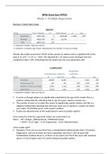
ANOVAa
Model Sum of Squares df Mean Square F Sig.
1 Regression 10871,964 3 3623,988 17,066 ,000b
Residual 48202,790 227 212,347
Total 59074,754 230
a. Dependent Variable: Salary per Day (£)
b. Predictors: (Constant), Age (Years), Attractiveness (%), Number of Years as a Model
Overall, the model accounts for 18.4% of the variance in saleries and is a signifcant ft to the
data (F (3, 227) = 17.07, p < .001). The adjusted R2 (.17) shows some shrinkage from the
unadjusted value (.184), indicatng that the model may not cross-generalize well.
Coefficientsa
Standardized
Unstandardized Coefficients Coefficients
Model B Std. Error Beta t Sig.
1 (Constant) -60,890 16,497 -3,691 ,000
Attractiveness (%) -,196 ,152 -,083 -1,289 ,199
Number of Years as a Model -5,561 2,122 -,548 -2,621 ,009
Age (Years) 6,234 1,411 ,942 4,418 ,000
a. Dependent Variable: Salary per Day (£)
It seems as though salaries are signifcantly predicted by the age of the model. This is a
positve relatonship (ß), indicatng that as age increases, salaries increase too.
The number of years as a model also seems to signifcantly predict salaries, but this is a
negatve relatonship indicatng that the more years you’ve spend as a model, the lower
your salary. This fnding seems a bit counter-intuitve.
Finally, the atractveness of the model doesn’t seem to predict salaries.
If we wanted to write the regression model, we could write it as:
Salary = ß0 + ß1Agei + ß2Experiencei + ß3Atractvenessi
= -60.89 + (6.23*Age) – (5.56*Experience) – (0.02*Atractveness)
Is this model valid?
Residuals: There are six cases that have a standardized residual greater than 3 (Casewise
Diagnostcs), and two of these are fairly substantal. We have 5.19% of cases with
standardized residuals above 2, so that’s as we expect, but 3% of the cases with residuals
above 2.5 (we’d expect only 1%), which indicates possible outliers.
, Normality of errors: The histogram reveals a skewed distributon, indicatng that the
normality of errors assumpton has been broken. The normal P-P plot verifes this
because the dashed line deviates considerably from the straight line, which indicates
what you’d get from normally distributed errors.
Homoscedastcity and independence of errors: The scaterplot of ZPREd vs. ZRESID does
not show a random patern. There is a distnct funneling, indicatng heteroscedastcity.
Multcollinearity: For the age and experience variables in the model, VIF values above 10
(or alternatvely, tolerance values are all well below 0,2), indicatng multcollinearity in
the data. In fact, the correlaton between these two variables is around .9, so these two
are measuring very similar things. Of course, this makes perfect sense because the older
the model is, the more years she would’ve spent modelling. This also explains the weird
result that the number of years spent modelling negatvely predicted salary: if you did a
simple regression with experience as the only predictor of salary you’ll fnd it has the
expected positve relatonship. This hopefully demonstrates why multcollinearity can
bias the regression model.
All in all, several assumptons have not been met and so this model is probably fairly
unreliable.
Exercise 2: Multple regression with categorical predictors
Dummy variables: a way of representng groups of people using only zeros and ones.
There are eight basis steps recoding a dummy:
1. Count the number of groups you want to recode and subtract 1.
2. Create as many new variables (dummy variables) as the value you calculated.
3. Choose one of your groups as a baseline against which all other groups will be
compared. Normally you’d pick the control group, or, if you don’t have a specifc
hypothesis, the group that represents your majority of people.
4. Having chosen a baseline group, assign that group values of 0 for all of your dummy
variables.
5. For your frst dummy variable, assign the value 1 to the frst group that you want to
compare against the baseline group. Assign all other groups 0 for this variable.
6. For the second dummy variable assign the value 1 to the second group that you want
to compare against the baseline group. Assign all other groups 0 for this variable.
7. Repeat this process untl you run out of dummy variables.
8. Place all of your dummy variables into the regression analysis In the same block.
Glastonbury Festval
There will be three dummy variables (one less than the number of groups).
The baseline group will be ‘no musical afliaton’o we give this group a code of 0 for all of
our dummy variables.
For our frst dummy variable, we could look at the ‘crusty’ group, and to do this we give
anyone who was a crusty a code of 1, and everyone else a code of 0.
- Recode into diferent variables.
- Name: Crusty -> change.
- Old and new values:
o Old value = 3o new value = 1.
o All other values = 0.
, For our second dummy variable, we could look at the ‘metaller’ group, and to do this we
give anyone who was a metaller a code of 1, and everyone else a code of 0.
- Recode into diferent variables.
- Name: Metaller -> change.
- Old and new values:
o Old value = 2o new value = 1.
o All other values = 0.
Our fnal dummy variable will code the ‘indie kid’ category. To do this, we give anyone
who was an indie kid a code of 1, and everyone else a code of 0.
- Recode into diferent variables.
- Name: Indie_Kid
- Old and new values:
o Old value = 1o new value = 1.
o All other values = 0.
Exercise 3: Happiness among the elderly
1. Assumpton of no outliers in:
a. X-space (Mahalanobis distances): maximum of Mahalanobis is 19, so the
assumpton is not met.
b. Y-space (Standardized residuals): nothing more extreme then -3 or +3, so the
assumpton is met.
c. XY-space (Cook’s distance): smaller then 0, so the assumpton is met.
2. Assumpton of an absence of multcollinearity:
a. Tolerance: assumpton is met.
3. Is the assumpton of homoscedastcity met?
a. Yes.
4. Is the assumpton of normally distributed residuals met?
a. Yes.
5. Is the assumpton of linearity met for the predictors Support of children and Support
of spouse? Use scater plots.
a. Support of children: not met.
b. Support of spouse: met.
Exercise 4: Happiness among the elderly (2)
1. Is age a signifcant predictor of happiness among the elderly? Does the additon of
years of educaton provide a signifcantly beter predicton of happiness among
elderly people than just age? Note. When an additonal variable is added to the
analysis, the assumptons actually should be checked again.
2. Does the additon of support by children and support by spouse signifcantly add to
the predicton of happiness among elderly people, if the efects of age and years of
educaton are already accounted for?
Exercise 5: Happiness among the elderly (3)
For this exercise, you need the same dataset as for exercise 3: the LifeSat.sav dataset.
In this analysis, a model with only support of spouse as a predictor of happiness among the
elderly is taken as a startng point. The main queston is whether the additon of socio-
economic economic status to this model leads to a signifcantly beter predicton.
, In SPSS, perform the analysis required to answer the following queston:
Does the additon of socio-economic economic status signifcantly add to the predicton of
happiness among elderly people, if the efect of support of spouse is already accounted for?
Use the group with low socio-economic status as the reference group.
The syntax of the analyses of exercises 3 to 5 can be found on Blackboard.
Week 2. Moderaton and mediaton
Moderaton (model number 1)
Moderaton can involve an interacton between two contnuous variables, interacton
between a categorical and a contnuous variable, or an interacton between two categorical
variables.
Output 1. Main moderaton analysis
Moderaton is shown up by a signifcant interacton efect, and in this case the interacton is
highly signifcant, b = 0.105, 95% CI [0.047, 0.164], t = 3.57, p < .01, indicatng that the
relatonship between atractveness and support is moderated by gender.
Output 2. Interpret the moderaton eeect by examining the simple slopes
The table shows us the results of two diferent regressions: the regression for atractveness
as a predictor for support when the value for gender is:
Voordelen van het kopen van samenvattingen bij Stuvia op een rij:
√ Verzekerd van kwaliteit door reviews
Stuvia-klanten hebben meer dan 700.000 samenvattingen beoordeeld. Zo weet je zeker dat je de beste documenten koopt!
Snel en makkelijk kopen
Je betaalt supersnel en eenmalig met iDeal, Bancontact of creditcard voor de samenvatting. Zonder lidmaatschap.
Focus op de essentie
Samenvattingen worden geschreven voor en door anderen. Daarom zijn de samenvattingen altijd betrouwbaar en actueel. Zo kom je snel tot de kern!
Veelgestelde vragen
Wat krijg ik als ik dit document koop?
Je krijgt een PDF, die direct beschikbaar is na je aankoop. Het gekochte document is altijd, overal en oneindig toegankelijk via je profiel.
Tevredenheidsgarantie: hoe werkt dat?
Onze tevredenheidsgarantie zorgt ervoor dat je altijd een studiedocument vindt dat goed bij je past. Je vult een formulier in en onze klantenservice regelt de rest.
Van wie koop ik deze samenvatting?
Stuvia is een marktplaats, je koop dit document dus niet van ons, maar van verkoper bcrose. Stuvia faciliteert de betaling aan de verkoper.
Zit ik meteen vast aan een abonnement?
Nee, je koopt alleen deze samenvatting voor €3,49. Je zit daarna nergens aan vast.