Course Structure:
→ three weeks, 6 lectures and 6 tutorials
→ exam week: on campus exam on February 3rd, alongside a written assignment which is due on the
same day.
→ Additional tutorials after Thursday lectures if needed (sign up is necessary)
→ lecture recordings are available at the end of each week
→ weekly tutorial tasks and readings to do, datasets in SPSS exercises are on canvas.
Course Content:
→ Linear regression and correlation
→ Multivariate relationships
→ Multiple regression with (interactions)
General Course Remarks:
→ very fast paced course, and the content is cumulative
→ The material can be seen as abstract and complex, but you don't need to be insane at math
→ 40 Hours Per Week!
Multiple Regression Analysis: statistical method that shows the relationship between two or more
variables, this is usually expressed in a graph, and the method tests the relation between a dependent and
independent variable.
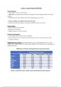
,What could cause these differences in hourly earnings between men and women:
→ individual preferences, which leaf to occupational and sectoral segregation
→ discrimination in the workplace
→ institutional arrangements in a given nation such as gender equality policy, childcare policy, marital,
unpaid leave etc.
→ multiple regression analysis can help us to figure out what the relationships between an outcome
and an explanatory variable are, while also taking the effects of all other (although there may be some
which are not identified) into account.
→ at the end of this course, we will possess the skill set to analyze and understand multi causal
phenomena
Linear Relationship and Linear Models: a linear relationship is a relationship between x and y, for
example hours of study and your grade, as hours of study increase, you expect your overall grade to increase
as well, hence a linear relationship which is positive.
→ Linear relationships are in straight lines, and the formula of this straight line is denoted by the
function 𝑦 = 𝛼 + 𝛽𝑥
→ This expresses the value on the y axis as a linear function of the values on the x-axis, and forms a
straight line with a slope, and a y intercept, also known as the alpha value.
Slope: a number that indicates how much the value of y increases, or decreases, with an increase of 1.0 of
x.
α/y intercept: a number that indicates where the line crosses the y axis, people also refer to this as the
constant.
,Statistical Model and Least Squares Prediction Equation: models are approximations of reality, and a
statistical model approximates a characteristic of individuals within a population.
→ everybody in a population has an age, but for large populations, this is time-consuming, a
mean/average age is displayed instead.
→ Relationships between two or more variables can also be expressed through the use of models, and
it can be represented as a linear function as shown above, you may also refer to this as a linear model.
Estimating a Line Based on Observed Data Points: we want to find the straight line that summarizes the
data in the most accurate way, the best way, but how do we do that?
→ we make use of a prediction equation: : 𝑦̂ = 𝑎 + 𝑏𝑥
→ y hat is the predicted value of y given by the value of x, where we must also calculate the y intercept
and slope with the following…
→ The slope also represents the strength of a relationship between x and y, or the effect that x has on
y directly.
→ The formula for this is the covariance of x and y, divided by the variance of x, the covariance of x
and y expressed only in units of x.
Most Important Property of the Prediction Equation: it has the least squares property.
→ you want the best matching or fitting line to the cloud of data points, but how do you find that?
→ it is the line where the distance between the predicted values for y, and their observed value, is the
smallest, thus being most accurate.
→ the better the equation, the fewer residuals/errors there are
How To Summarise Size of Residuals?
→ by summing up their squared values, such as computing the sum of squared errors, an SSE.
→ The SSE is a measure of the discrepancy between the line 𝑦̂ = a +bx and the cloud of observed data
points
→ This prediction line 𝑦̂ = a +bx is also referred to as the least square line, as it is the one with the smallest
sum of squared errors.
, Residual: (𝑦𝑖 − 𝑦̂)2
→ The smaller the SSE, the better the line fits the dataset.
Recap This Lecture:
→ A linear function represents a straight line: y = α + βx
→ The prediction equation represents a collection of data points as a straight line: ŷ= a + bx
→ To get the prediction equation we need to calculate the a and b coefficients.
→ The prediction equation has the least squares property. This property will guarantee the best fitting
straight line to the data.
→ The least squares property is expressed with the Sum of Squared Errors = SSE. The SSE indicates the
discrepancy between the model and the data.
→ The SSE has a value that cannot be interpreted meaningfully
Linear Regression Model: y = a + bx
→ deterministic model, however this is a bit unrealistic in
social sciences, we use a probabilistic model instead, which
allows for variability in y at each given value of x, a
conditional distribution.
→ In probabilistic model, 𝛼 + 𝛽𝑥 represents the mean of the
conditional distribution of y-values rather than y itself
→ The linear regression function can be shown as: 𝐸(𝑦) =
𝛼 + 𝛽𝑥
→ This function describes how the mean of a dependent (response/outcome) variable changes in
accordance with the value of the independent (explanatory/predictor) variable
This: 𝐸(𝑦) = 𝛼 + 𝛽𝑥 represents…
→ E(y) is the mean of the conditional distribution of y
→ E stands for expected value, means nothing more than the mean
→ Alpha is the intercept (where the y-axis is crossed, also called constant, y when x is 0)
→ Beta is the slope of your variable of intest
→ x is the specific value of your beta variable if you are using this as a prediction
Additionally…
Voordelen van het kopen van samenvattingen bij Stuvia op een rij:
√ Verzekerd van kwaliteit door reviews
Stuvia-klanten hebben meer dan 700.000 samenvattingen beoordeeld. Zo weet je zeker dat je de beste documenten koopt!
Snel en makkelijk kopen
Je betaalt supersnel en eenmalig met iDeal, Bancontact of creditcard voor de samenvatting. Zonder lidmaatschap.
Focus op de essentie
Samenvattingen worden geschreven voor en door anderen. Daarom zijn de samenvattingen altijd betrouwbaar en actueel. Zo kom je snel tot de kern!
Veelgestelde vragen
Wat krijg ik als ik dit document koop?
Je krijgt een PDF, die direct beschikbaar is na je aankoop. Het gekochte document is altijd, overal en oneindig toegankelijk via je profiel.
Tevredenheidsgarantie: hoe werkt dat?
Onze tevredenheidsgarantie zorgt ervoor dat je altijd een studiedocument vindt dat goed bij je past. Je vult een formulier in en onze klantenservice regelt de rest.
Van wie koop ik deze samenvatting?
Stuvia is een marktplaats, je koop dit document dus niet van ons, maar van verkoper ollied. Stuvia faciliteert de betaling aan de verkoper.
Zit ik meteen vast aan een abonnement?
Nee, je koopt alleen deze samenvatting voor €10,49. Je zit daarna nergens aan vast.