Production functions
● Production functions refer to the conversion process (inputs to outputs)
● Shows the maximum a firm can produce using various combinations of inputs
○ Inputs are used as efficiently as possible and there is no waste
● Assume 2 inputs Q = F(K,L) and that Q is concave and monotonic
Short-run / 1 input model
● In the short run, one factor of production is fixed - Q = F(L)
● The producer’s choice set of production plans are technologically feasible
○ Increasing MPL implies non-convexity
● The production function is the set of production plans with no waste of inputs
● There is diminishing marginal returns as labour increases
Marginal and average product
● Marginal product of labour - additional output produced by one more worker
○ = change in total product / change in quantity of labour
○ A linear production function has a constant MPL
○ Assume diminishing marginal productivity
○ MPL = the slope of the production function
● The average product of labour = total product / quantity of labour
● Maximum output occurs when MP = 0
● The peak of MP is where diminishing marginal returns begin
● If MPL > APL, the average is rising
● If APL > MPL, the average is falling
● Negative MPL implies a downward sloping production frontier
Isoquants
● Isoquants show all combinations of labour and capital that produce a given
level of output
● They are downward sloping, monotonic, thin, convex and do not cross
● They represent output (measurable)
● They arise from production functions (tech constraints faced by producers)
● Doubling inputs alters the production technology - producing 2x as much
output as before (returns to scale)
The marginal rate of technical substitution
● The 𝑀𝑅𝑇𝑆𝐿,𝐾 (of labour for capital) is the slope of the isoquant
○ Diminishes as you move down the isoquant
● Differentiate the production function to find the MRTS
, 𝑀𝑃
○ 𝑀𝑅𝑇𝑆𝐿,𝐾 = 𝑀𝑃 𝐿
𝐾
● Shows how many units of capital the firm can substitute for one unit of labour
whilst keeping output constant
Returns to scale (long-run)
● Returns to scale = % △ in output / % △ in inputs
● 𝑓(𝑡𝐾, 𝑡𝐿) = 𝑡 𝑘 𝑓(𝐾, 𝐿) = 𝑡𝑄(homogeneous production function)
● 𝑓(𝐾, 𝐿) = 𝐴𝐿𝑎 𝐾 𝑏
○ K or a+b >1 = increasing returns
○ K or a+b =1 = constant returns
○ K or a+b <1 = decreasing returns
● Isoquants are radial expansions of one another
○ Constant returns to scale production functions are homothetic
○ MRTS depends on the ratio of K to L - not on the scale of production
Returns to scale and diminishing marginal product
● Can have diminishing returns to labour but constant returns to scale
● 𝑓(𝐿, 𝐾) = 𝐿𝑎 𝐾 𝑏
○ 𝑀𝑃𝐿 = 𝑎𝐿𝑎−1 𝐾 𝑏 and 𝑀𝑃𝐾 = 𝑏𝐿𝑎 𝐾 𝑏−1
● There is diminishing marginal product if
○ 𝑎(𝑎 − 1)𝐿𝑎−2 𝐾 𝑏 < 0(differential of MPL)
○ 𝑏(𝑏 − 1)𝐿𝑎 𝐾 𝑏−2 < 0(differential of MPK)
● If the exponents 0 < a, b < 1, the MPL and MPK will be diminishing
● 𝑓(𝐿, 𝐾) = 𝐴𝐿𝑎 𝐾 𝑏
○ B < 1 shows diminishing marginal product
○ B > 1 shows increasing marginal product
○ a+b>1 shows IRS
Linear production functions
● Q = f(L,H) = aL + bH
● MRTS = -a/b (constant along linear isoquants)
Fixed proportion production functions
● Q= f(L,H) = min (aH + bO)
● If aH<BO, then Q=aH and H is the binding constraint
● If aH=bO, then both inputs are fully utilised
Cobb Douglas production function
● 𝑄 = 𝐴𝐿𝑎 𝐾 𝑏
● lnQ = lnA + alnL + blnK - linear in logarithms
○ a is the elasticity of output with respect to L
○ b is the elasticity of output with respect to K


