Correlation research methods 2022-2023
Week 1
Different aspects of empirical research
‣ Samples versus populations
‣ Descriptive or inferential statistics
‣ Levels of measurement
‣ Experimental, quasi-experimental or correlational method
There is different kinds of sampling.
Firstly, there is simple random
sampling for which every member in a
population has an equal chance to be
sampled. Then there is stratified
sampling where a population is divided
into strata based on descriptive factors
such as age and gender. A random
sample is then drawn from each
sample. Lastly, there is convenience sampling which is a sample technique using
people who are readily available.
Descriptive statistics summarizes data with a mean, median, mode, variance, and
standard deviation after studying the sample. For inferential statistics we use a sample
to create generalizability for the population we drew the sample from. Procedures used
to do this are null hypothesis testing and confidence interval estimation. Null
hypothesis testing first formulates a null and alternative hypothesis. Then a decision
rule is made and after that the t- and p-value are obtained. Based on these values the
null hypothesis is kept or rejected.
In this course categorical and quantitative variables are distinguished. Categorical
examples are gender, diagnosis, social class, etc. examples of quantitative variables are
age, IQ, exam scores, etc.
Pearson’s correlation coefficient is a coefficient in statistics that measures the
statistical relationship, or association, between two continuous variables. If r = 0 there is
no linear association but there might be a non-linear one.
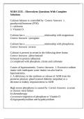
Rule of thumb table for association
r Interpretation correlational strength
1.00 Perfect
0.50 Strong
0.30 Medium
0.10 Small
0.00 No effect
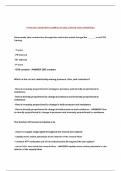
When doing a data analysis a scatterplot is made in which outliers can be seen.
Outliers are data marks that don’t lie within the line of association. Bivariate outlies are
values that are not atypical for the distributions of variables x and y considered
separately, but is atypical for their bivariate distribution.
, t=r
√ N −2
1−r 2
The p-value is the probability of the data in the sample. When p<α reject the null
hypothesis.
Week 2
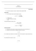
X and Y are linearly correlated and their relation is drawn by
drawing a straight line through the scatterplot.
r 2XY = proportion of the variance in X you can linearly predict from
Y
Correlation ≠ causation
There are different types of relationships between variables
‣ Direct: X Y
‣ Indirect: X Z (mediator) Y
‣ Spurious: X Z (mediator) Y
‣ Correlation coefficient: X1 ↔ X2
In simple linear regression there’s an independent variable X and a dependent variable
Y. The arrow always points to the dependent variable (X Y).
A linear relationship between Y and X means that we can predict Y from X using a
'
linear function. We use the formula: Y =b 0+ b1 X . Y ' is the predicted value of Y given X .
b 0 is the intercept which means the predicted value Y ' when someone scores 0 on X .
b 1 is the regression coefficient which is the change in Y ' when X increases with one
unit. b 0 and b 1 are the parameters of the model.
Simple regression analysis step by step
1. Find the best fitting straigt line given all the values in the data set. The values
from which you can best predict Y from X.
2. Decide how well Y can be predicted by inspecting individual prediction errors
using the formula: e 1=Y i−Y i ' .
3. Check whether you can generalize the results to the population levels.
Sy
b 1=r
Sx
Σ (Z x × Z y )
r= where Z x =( X −X ) / S x and Z y =( Y −Y ) / S y
N
2 2 2
The total variance can be split into two parts SY =SY ' + S e . To calculate the proportion of
2
2 SY ' 2
explained variance we use RY ∙ X = 2 . 1−R Y ∙ X is the unexplained variance.
SY
b^1−b1
t=
SE ( b^ )
1
Week 1
Different aspects of empirical research
‣ Samples versus populations
‣ Descriptive or inferential statistics
‣ Levels of measurement
‣ Experimental, quasi-experimental or correlational method
There is different kinds of sampling.
Firstly, there is simple random
sampling for which every member in a
population has an equal chance to be
sampled. Then there is stratified
sampling where a population is divided
into strata based on descriptive factors
such as age and gender. A random
sample is then drawn from each
sample. Lastly, there is convenience sampling which is a sample technique using
people who are readily available.
Descriptive statistics summarizes data with a mean, median, mode, variance, and
standard deviation after studying the sample. For inferential statistics we use a sample
to create generalizability for the population we drew the sample from. Procedures used
to do this are null hypothesis testing and confidence interval estimation. Null
hypothesis testing first formulates a null and alternative hypothesis. Then a decision
rule is made and after that the t- and p-value are obtained. Based on these values the
null hypothesis is kept or rejected.
In this course categorical and quantitative variables are distinguished. Categorical
examples are gender, diagnosis, social class, etc. examples of quantitative variables are
age, IQ, exam scores, etc.
Pearson’s correlation coefficient is a coefficient in statistics that measures the
statistical relationship, or association, between two continuous variables. If r = 0 there is
no linear association but there might be a non-linear one.
Rule of thumb table for association
r Interpretation correlational strength
1.00 Perfect
0.50 Strong
0.30 Medium
0.10 Small
0.00 No effect
When doing a data analysis a scatterplot is made in which outliers can be seen.
Outliers are data marks that don’t lie within the line of association. Bivariate outlies are
values that are not atypical for the distributions of variables x and y considered
separately, but is atypical for their bivariate distribution.
, t=r
√ N −2
1−r 2
The p-value is the probability of the data in the sample. When p<α reject the null
hypothesis.
Week 2
X and Y are linearly correlated and their relation is drawn by
drawing a straight line through the scatterplot.
r 2XY = proportion of the variance in X you can linearly predict from
Y
Correlation ≠ causation
There are different types of relationships between variables
‣ Direct: X Y
‣ Indirect: X Z (mediator) Y
‣ Spurious: X Z (mediator) Y
‣ Correlation coefficient: X1 ↔ X2
In simple linear regression there’s an independent variable X and a dependent variable
Y. The arrow always points to the dependent variable (X Y).
A linear relationship between Y and X means that we can predict Y from X using a
'
linear function. We use the formula: Y =b 0+ b1 X . Y ' is the predicted value of Y given X .
b 0 is the intercept which means the predicted value Y ' when someone scores 0 on X .
b 1 is the regression coefficient which is the change in Y ' when X increases with one
unit. b 0 and b 1 are the parameters of the model.
Simple regression analysis step by step
1. Find the best fitting straigt line given all the values in the data set. The values
from which you can best predict Y from X.
2. Decide how well Y can be predicted by inspecting individual prediction errors
using the formula: e 1=Y i−Y i ' .
3. Check whether you can generalize the results to the population levels.
Sy
b 1=r
Sx
Σ (Z x × Z y )
r= where Z x =( X −X ) / S x and Z y =( Y −Y ) / S y
N
2 2 2
The total variance can be split into two parts SY =SY ' + S e . To calculate the proportion of
2
2 SY ' 2
explained variance we use RY ∙ X = 2 . 1−R Y ∙ X is the unexplained variance.
SY
b^1−b1
t=
SE ( b^ )
1