SPSS Sessies
Sessie 1
Opdracht 1
A. Make a scatter plot of skinfold thickness (LSKIN) (x-axis) and body mass (DEN) (y-axis).
In SPSS: Graphs – Legacy – Scatterplot – Simple scatter - variabelen toevoegen
Voor regressielijn door het plot heen: Dubbel klik op output – Add fit line at total – OK
B. Describe the relationship between skinfold and body mass:
De relatie is sterk (punten liggen dicht op de lijn), negatief (lijn loopt naar beneden) en lineair
(rechte lijn, geen gekke vormen).
C. Perform a regression analysis to predict body mass (DEN) from skinfold (LSKIN). What is the
regression equation? What is the value of R square and what does this mean?
In SPSS: Analyse – Regression – Linear – DEN als Dependent en LSKIN als Independent – OK
R square is .72. Dat betekent dat 72% van de variantie van de afhankelijke variabele, verklaart
wordt door de onafhankelijke variabele. Dit is een hoog percentage (>50%).
D. Formulate the hypotheses concerning the regression coefficient.
Hypotheses verwijzen altijd naar de populatie, vandaar dat we ook gebruik maken van de Griekse
cijfers die horen bij de populatie. Als we verwijzen naar een sample, gebruiken we de b-value. De
hypotheses die horen bij de regressie-coëfficiënt zijn als volgt:
H0: ß1 = 0
Ha: ß1≠ 0
, E. What is your conclusion concerning this hypotheses?
De regressie-coëfficiënt van LSKIN is significant (t(90) = -15.23, p < .01). Vanuit de b-waarde
kunnen we infereren dat een toename in skinfold thickness geassocieerd is met een afname in
bodymassa (b = -.06).
F. Redo the analysis and save (use the Save option) the predicted values for body mass. Look up
the new variable in the data editor.
In SPSS: Analyse – Regression – Linear – invullen variabelen – SAVE aanklikken – Predicted
Values: Unstandardized - OK
G. Make a scatter plot of skinfold thickness (LSKIN) (x-axis) and the predicted values for body
mass (y-axis). Compare this scatterplot to the one created in a. Explain the difference between
the two plot and include the term “residual” in this explanation.
In SPSS: Graphs – Legacy – Scatterplot – variabelen toevoegen
De voorspelde waarden zijn een lineaire combinatie van de onafhankelijke variabele en zijn dus
perfect gecorreleerd met deze variabele. De voorspelde waarden liggen op een rechte lijn, dat
wil zeggen de regressielijn. De waargenomen (lichaamsgewicht) waarden staan verspreid over
deze lijn. Hoe dichter de waargenomen waarden bij de lijn liggen, hoe beter de voorspelling.
Opdracht 2
A. Compute the correlations and regression coefficients for the 4 variable pairs X1-Y1 through X4-
Y4. What do you notice about these results?
In SPSS: Analyse – Correlate – Bivariate – alle variabelen toevoegen – OK.
Uit de tabel blijkt dat alle paren correleren met .816.
In SPSS: Analyse – Regression.
Wanneer we een regressieanalyse uitvoeren voor de verschillende paren, blijkt dat de b-waarde
voor elk paar gelijk is: b = .50
Sessie 1
Opdracht 1
A. Make a scatter plot of skinfold thickness (LSKIN) (x-axis) and body mass (DEN) (y-axis).
In SPSS: Graphs – Legacy – Scatterplot – Simple scatter - variabelen toevoegen
Voor regressielijn door het plot heen: Dubbel klik op output – Add fit line at total – OK
B. Describe the relationship between skinfold and body mass:
De relatie is sterk (punten liggen dicht op de lijn), negatief (lijn loopt naar beneden) en lineair
(rechte lijn, geen gekke vormen).
C. Perform a regression analysis to predict body mass (DEN) from skinfold (LSKIN). What is the
regression equation? What is the value of R square and what does this mean?
In SPSS: Analyse – Regression – Linear – DEN als Dependent en LSKIN als Independent – OK
R square is .72. Dat betekent dat 72% van de variantie van de afhankelijke variabele, verklaart
wordt door de onafhankelijke variabele. Dit is een hoog percentage (>50%).
D. Formulate the hypotheses concerning the regression coefficient.
Hypotheses verwijzen altijd naar de populatie, vandaar dat we ook gebruik maken van de Griekse
cijfers die horen bij de populatie. Als we verwijzen naar een sample, gebruiken we de b-value. De
hypotheses die horen bij de regressie-coëfficiënt zijn als volgt:
H0: ß1 = 0
Ha: ß1≠ 0
, E. What is your conclusion concerning this hypotheses?
De regressie-coëfficiënt van LSKIN is significant (t(90) = -15.23, p < .01). Vanuit de b-waarde
kunnen we infereren dat een toename in skinfold thickness geassocieerd is met een afname in
bodymassa (b = -.06).
F. Redo the analysis and save (use the Save option) the predicted values for body mass. Look up
the new variable in the data editor.
In SPSS: Analyse – Regression – Linear – invullen variabelen – SAVE aanklikken – Predicted
Values: Unstandardized - OK
G. Make a scatter plot of skinfold thickness (LSKIN) (x-axis) and the predicted values for body
mass (y-axis). Compare this scatterplot to the one created in a. Explain the difference between
the two plot and include the term “residual” in this explanation.
In SPSS: Graphs – Legacy – Scatterplot – variabelen toevoegen
De voorspelde waarden zijn een lineaire combinatie van de onafhankelijke variabele en zijn dus
perfect gecorreleerd met deze variabele. De voorspelde waarden liggen op een rechte lijn, dat
wil zeggen de regressielijn. De waargenomen (lichaamsgewicht) waarden staan verspreid over
deze lijn. Hoe dichter de waargenomen waarden bij de lijn liggen, hoe beter de voorspelling.
Opdracht 2
A. Compute the correlations and regression coefficients for the 4 variable pairs X1-Y1 through X4-
Y4. What do you notice about these results?
In SPSS: Analyse – Correlate – Bivariate – alle variabelen toevoegen – OK.
Uit de tabel blijkt dat alle paren correleren met .816.
In SPSS: Analyse – Regression.
Wanneer we een regressieanalyse uitvoeren voor de verschillende paren, blijkt dat de b-waarde
voor elk paar gelijk is: b = .50