Module I Summary: The Normal Distribution
1. NORMAL DISTRIBUTION BASICS
• = continuous, symmetrical, bell-shaped probability distribution.
o E.g. height of woman & men, weight of an apple…
• Notation (parameters of the normal distribution):
y ~ N(μ, σ)
o μ (mu) = population mean (expected value of ‘y)
▪ determine the centre so thereby the position of the curve
▪ moat, mean & the medium of the normal distribution
o σ (sigma) = population standard deviation
▪ determine shape of distribution: spread or width distribution
▪ e.g. the more apples differ in weight, the larger σ will be, the wider/larger
the normal distribution will be
• Example if a variable is normally distributed, we write:
o the weight of an apple is normal distributed: y N (µ, σ)
▪ notation ‘’ = ‘is distributed as’
▪ ‘N’ = ‘normal’
▪ Between ‘( …. )’ you write your parameters
2. PROPERTIES OF THE NORMAL DISTRIBUTION = GAUSSIAN DISTRIBUTION
• Symmetrical (50% left of the mean, 50% right) + bell-shaped & unimodal (1 peak,
highest at the mean - most of distribution at middle)
• ranging from minus infinity to infinity
• we are not interested in function itself but area under the curve (integral)!
• Area under the curve = 1 (represents total probability)
o The probability of (ex. a weight less than 100g) is represented
by a certain area under the curve (so it’s the probability that
a random picked apples weights 100g of less)
• Probability of an exact value (e.g. y = 175) = 0
o We calculate probabilities over intervals, e.g. P(170 < y <
180)
3. PROBABILITY DENSITY FUNCTION (PDF)
• To determine probabilities
o For continuous variables, area under the curve over an
interval = probability
• Formula
• Defines the shape of the curve.
• Can't compute the area with simple formulas → use numerical methods, tables, or
software
1
,4. STANDARD NORMAL DISTRIBUTION
• Denoted: z ~ N(0, 1)
o Mean = 0, SD = 1
o Standard deviation following standard normal distribution = usually denoted with
‘z’ rather then ‘y’
• Use z-scores to convert any normal distribution to standard normal distribution:
→ z-value 'z' indicates the number of standard deviations that the y value is
away from the mean of variable y.
5. EMPIRICAL RULE (68–95–99.7 RULE)
• Useful for estimating probabilities without exact calculation
(‘quick summary normal distribution’)
• show how much of the distribution (how much of the area
under the curve) is between certain thresholds.
• ~68% of values within ±1σ
• ~95% of values within ±2σ
• ~99.7% of values within ±3σ
• Example: If μ = 69, σ = 2.5
→ 95% fall between 64.0 and 74.0
6. VISUALIZING NORMALITY
• Histogram: shows if distribution is bell shaped
o Note every normal distribution is bell-shaped!
• Boxplot: Shows symmetry, spread, outliers
o Quick check if distribution is symmetric but there are many other distributions
that also are symmetric
• QQ-Plot: Best tool to test normality → if data follow a straight line = likely normal
Boxplot QQ-plot
7. DISCRETE DISTRIBUTIONS
• Discrete variables = variables that can take only specific, separate values (e.g.,
integers)
o Probability of a single outcome is non-zero (unlike in continuous distributions).
• Unlike continuous distributions (which use a density function), discrete distributions use
a probability mass function (PMF)
• sum of all probabilities of discrete outcomes is always 1
2
, • example 1: throwing a fair die:
o Possible outcomes: 1, 2, 3, 4, 5, 6
o Probability of each outcome: 1/6
• example 1: Tossing two dice and summing the result:
• Outcomes range from 2 to 12
• Some outcomes (like 7) are more likely than others
(like 2 or 12)
8. COMMON POPULATION PARAMETERS:
• Mean (μ) = average of all values in a population
• Standard deviation (σ) = measures the spread of values around the mean.
• Variance (σ²) = square of the standard deviation; quantifies variability.
• Mode = most frequently occurring value.
• Median = middle value when data is sorted.
• Range = difference between the highest and lowest values.
• Interquartile Range (IQR ) = range between the 25th and 75th percentile; shows middle
50% of data.
9. IMPORTANT CONCEPTS:
• Population parameters describe entire populations but are usually unknown in
practice.
• We often work with samples, so we use estimators to approximate these parameter
• Estimators from Samples:
o Sample Mean (ȳ) estimates Population Mean (μ)
o Sample Standard Deviation (s) estimates σ
o Sample Variance (s²) estimates σ²
• Notation Tip:
o Greek letters (μ, σ) = population parameters
o Latin letters with bars or hats (ȳ, s²… ) = sample estimates
3
, MODULE 2: Hypothesis Testing (One-Sample t-Test)
Purpose
To determine if there is enough evidence from a sample to infer something about a
population mean
Example: we want to say something about whole population (e.g. all people of NLs) but measuring
whole population is usually impossible, so we measure a representative sample, & try to interfere
from that sample something about the population.
Statistics are invented to carry the results from the sample up to the population, taking into
account that, just by chance, samples may have means, proportions,or standard deviations that
differ somewhat from the population as a whole. We:
1. Make an initial assumption (of no effect = H0)
2. Collect evidence In the sample
3. Decide, based on the evidence, to reject or not reject the initial assumption
Our initial assumption of ‘no effect’ is called null-hypothesis H0.
It is contrasted with the alternative hypothesis Ha. We can use a courtroom analogy:
H0: defendant is not guilty
Ha: defendant is guilty
➔ ‘the jury’ gives the defendant the benefit of the doubt, unless the evidence is
‘overwhelming
The hypothesis test needs a test statistic, a value we can compute to see how far away our
results in the sample are from the null hypothesis. We want to quantify the evidence against
innocence. In t-tests, this is the t-test statistic.
For a one-sample test of the mean, say H0 μ= 100g, vs (for example) Ha μ ≠100g,
➔ 𝑡 = (𝑦̅ − 100) /𝑠𝑒(𝑦̅ )
➔ If null hypothesis = true, we expect a t-value close to zero
➔ But how large or small can this value get in our sample just by chance? The The 0-
distribution of the test statistic can tell us that. The exact shape of the distribution is given
by the degrees of freedom that are in the sample data. For the one-sample t-test, we
have: Test statistic ~ tdf=n-1. (The symbol ~ means 'is distributed as ...', n = the sample
size)
4
1. NORMAL DISTRIBUTION BASICS
• = continuous, symmetrical, bell-shaped probability distribution.
o E.g. height of woman & men, weight of an apple…
• Notation (parameters of the normal distribution):
y ~ N(μ, σ)
o μ (mu) = population mean (expected value of ‘y)
▪ determine the centre so thereby the position of the curve
▪ moat, mean & the medium of the normal distribution
o σ (sigma) = population standard deviation
▪ determine shape of distribution: spread or width distribution
▪ e.g. the more apples differ in weight, the larger σ will be, the wider/larger
the normal distribution will be
• Example if a variable is normally distributed, we write:
o the weight of an apple is normal distributed: y N (µ, σ)
▪ notation ‘’ = ‘is distributed as’
▪ ‘N’ = ‘normal’
▪ Between ‘( …. )’ you write your parameters
2. PROPERTIES OF THE NORMAL DISTRIBUTION = GAUSSIAN DISTRIBUTION
• Symmetrical (50% left of the mean, 50% right) + bell-shaped & unimodal (1 peak,
highest at the mean - most of distribution at middle)
• ranging from minus infinity to infinity
• we are not interested in function itself but area under the curve (integral)!
• Area under the curve = 1 (represents total probability)
o The probability of (ex. a weight less than 100g) is represented
by a certain area under the curve (so it’s the probability that
a random picked apples weights 100g of less)
• Probability of an exact value (e.g. y = 175) = 0
o We calculate probabilities over intervals, e.g. P(170 < y <
180)
3. PROBABILITY DENSITY FUNCTION (PDF)
• To determine probabilities
o For continuous variables, area under the curve over an
interval = probability
• Formula
• Defines the shape of the curve.
• Can't compute the area with simple formulas → use numerical methods, tables, or
software
1
,4. STANDARD NORMAL DISTRIBUTION
• Denoted: z ~ N(0, 1)
o Mean = 0, SD = 1
o Standard deviation following standard normal distribution = usually denoted with
‘z’ rather then ‘y’
• Use z-scores to convert any normal distribution to standard normal distribution:
→ z-value 'z' indicates the number of standard deviations that the y value is
away from the mean of variable y.
5. EMPIRICAL RULE (68–95–99.7 RULE)
• Useful for estimating probabilities without exact calculation
(‘quick summary normal distribution’)
• show how much of the distribution (how much of the area
under the curve) is between certain thresholds.
• ~68% of values within ±1σ
• ~95% of values within ±2σ
• ~99.7% of values within ±3σ
• Example: If μ = 69, σ = 2.5
→ 95% fall between 64.0 and 74.0
6. VISUALIZING NORMALITY
• Histogram: shows if distribution is bell shaped
o Note every normal distribution is bell-shaped!
• Boxplot: Shows symmetry, spread, outliers
o Quick check if distribution is symmetric but there are many other distributions
that also are symmetric
• QQ-Plot: Best tool to test normality → if data follow a straight line = likely normal
Boxplot QQ-plot
7. DISCRETE DISTRIBUTIONS
• Discrete variables = variables that can take only specific, separate values (e.g.,
integers)
o Probability of a single outcome is non-zero (unlike in continuous distributions).
• Unlike continuous distributions (which use a density function), discrete distributions use
a probability mass function (PMF)
• sum of all probabilities of discrete outcomes is always 1
2
, • example 1: throwing a fair die:
o Possible outcomes: 1, 2, 3, 4, 5, 6
o Probability of each outcome: 1/6
• example 1: Tossing two dice and summing the result:
• Outcomes range from 2 to 12
• Some outcomes (like 7) are more likely than others
(like 2 or 12)
8. COMMON POPULATION PARAMETERS:
• Mean (μ) = average of all values in a population
• Standard deviation (σ) = measures the spread of values around the mean.
• Variance (σ²) = square of the standard deviation; quantifies variability.
• Mode = most frequently occurring value.
• Median = middle value when data is sorted.
• Range = difference between the highest and lowest values.
• Interquartile Range (IQR ) = range between the 25th and 75th percentile; shows middle
50% of data.
9. IMPORTANT CONCEPTS:
• Population parameters describe entire populations but are usually unknown in
practice.
• We often work with samples, so we use estimators to approximate these parameter
• Estimators from Samples:
o Sample Mean (ȳ) estimates Population Mean (μ)
o Sample Standard Deviation (s) estimates σ
o Sample Variance (s²) estimates σ²
• Notation Tip:
o Greek letters (μ, σ) = population parameters
o Latin letters with bars or hats (ȳ, s²… ) = sample estimates
3
, MODULE 2: Hypothesis Testing (One-Sample t-Test)
Purpose
To determine if there is enough evidence from a sample to infer something about a
population mean
Example: we want to say something about whole population (e.g. all people of NLs) but measuring
whole population is usually impossible, so we measure a representative sample, & try to interfere
from that sample something about the population.
Statistics are invented to carry the results from the sample up to the population, taking into
account that, just by chance, samples may have means, proportions,or standard deviations that
differ somewhat from the population as a whole. We:
1. Make an initial assumption (of no effect = H0)
2. Collect evidence In the sample
3. Decide, based on the evidence, to reject or not reject the initial assumption
Our initial assumption of ‘no effect’ is called null-hypothesis H0.
It is contrasted with the alternative hypothesis Ha. We can use a courtroom analogy:
H0: defendant is not guilty
Ha: defendant is guilty
➔ ‘the jury’ gives the defendant the benefit of the doubt, unless the evidence is
‘overwhelming
The hypothesis test needs a test statistic, a value we can compute to see how far away our
results in the sample are from the null hypothesis. We want to quantify the evidence against
innocence. In t-tests, this is the t-test statistic.
For a one-sample test of the mean, say H0 μ= 100g, vs (for example) Ha μ ≠100g,
➔ 𝑡 = (𝑦̅ − 100) /𝑠𝑒(𝑦̅ )
➔ If null hypothesis = true, we expect a t-value close to zero
➔ But how large or small can this value get in our sample just by chance? The The 0-
distribution of the test statistic can tell us that. The exact shape of the distribution is given
by the degrees of freedom that are in the sample data. For the one-sample t-test, we
have: Test statistic ~ tdf=n-1. (The symbol ~ means 'is distributed as ...', n = the sample
size)
4