February 2025, by Isabel Rutten
Content
Unit 1: Introduction to Decision Modeling & Linear Programming .......................................... 2
Unit 2: Sensitivity Analysis .................................................................................................... 3
Unit 3: Sensitivity Analysis (continued) & Binary Models ....................................................... 3
Unit 4: Sales & Marketing Applications .................................................................................. 4
Unit 5: Investment Portfolio Optimization............................................................................... 4
Unit 6: Investment Portfolio Optimization II............................................................................ 5
Examples .............................................................................................................................. 6
Printers (Unit 1) ................................................................................................................. 6
Brewery (Unit 1) ................................................................................................................ 6
TropiCo (Unit 1) ................................................................................................................. 6
ClosetCo (Unit 2) ............................................................................................................... 6
NordiCo (Unit 3) ................................................................................................................ 7
Influencers (Unit 3) ............................................................................................................ 7
Repsoil (Unit 3).................................................................................................................. 7
Cotton Market (Unit 4) ....................................................................................................... 8
Digital Marketing (Unit 4) ................................................................................................... 8
Invest (Unit 5) .................................................................................................................... 8
Vintage stocks (Unit 6) ...................................................................................................... 9
Excel ................................................................................................................................. 9
1
Systems Optimization – Summary. February 2025, by Isabel Rutten.
, Unit 1: Introduction to Decision Modeling & Linear
Programming
Decision-making model: structured process which can be used to guide managers to make
decisions. Developed in an iterative manner, through a four-step cycle:
1. Formulate: Develop a formal (mathematical) model of the given (real-world) decision.
2. Evaluate: Apply the decision model and produce a formal recommendation.
3. Interpret: Examine (computer) outcomes and determine a clear course of action.
4. Refine: Test possible decision model changes and find ways to improve the model.
If more analysis is needed, start again from step 1. Else, implement the decision.
Linear programming: mathematical modeling technique in which a linear objective function
is maximized or minimized when subjected to various constraints (represented by linear
equations or inequalities), used for quantitative decisions, aim to find optimum. Components:
- Decision variables: unknown quantities, we want to optimize this.
- Objective function: goal of decision-maker, two types: maximization or minimization
- Constraints: limitations on possible solutions of the problem (e.g. availability of
scarce resources). RHS (Right-Hand Side) is number located on RHS of constraint.
- Non-negativity conditions: special constraints which require all variables to be
either zero or positive
Assumptions of linear programming:
- Proportionality: the contribution of any decision variable to the objective function is
proportional to its value
- Additivity: e.g. total profit of objective function is determined by the sum of profit
contributed by each product separately
- Continuity: the decision variables are continuous (i.e. fractions are allowed)
- Certainty: all constant terms, objective function and constraints are known and will
not change
i.e. objective function and constraints must be linear w.r.t. decision variables.
Linear function: a function whose graph is a straight line and which is represented
by an equation of the form 𝑦 = 𝑎𝑥 + 𝑏.
Allowable variations: constraints can be ≤, ≥, or =; non-integer or integer coefficients
are allowed; negative or positive coefficients are allowed.
Graphical approach of linear programming (only if 2 dec vars):
1. Plot each of the constraints.
2. Determine the feasible region (satisfy all constraints).
3. Draw the objective function.
4. Determine the optimal solution.
Special cases of graphical approach:
- No feasible solutions: to satisfy one of the constraints, another must be violated
- Unbounded: value of the objective function can be increased without limit
- Redundant constraint: a constraint that does not form a unique boundary of the
feasible solution space, its removal would not alter the feasible solution space
- Multiple optimal solutions: different combinations of values of the decision
variables yield the same optimal value
2
Systems Optimization – Summary. February 2025, by Isabel Rutten.


