Discovering Statistics Using IBM SPSS Statistics
Chapter 1
Levels of measurement
Categorical (entities are divided into distinct categories):
- Nominal variable/categorical
• Binary (Only two values possible: Married, Pregnant, etc.)
• With more than two categories (e.g. whether someone is an omnivore, vegetarian, vegan, or
fruitarian)
- Ordinal variable: The same as a nominal variable but the categories have a logical order from
lower to higher, smaller to larger
-e.g. whether people got a fail, a pass, a merit or a distinction in their exam
-Answers to statements on a 5-point or 7-point scale are typically ordinal
Continuous (entities get a distinct score):
- Interval variable: Equal intervals on the variable represent equal differences in the property
being measured
-e.g. Temperature in degrees Celsius: the difference between 6 and 8 is the same as
the difference between 13 and 15
- Ratio variable: The same as an interval variable, but the ratios of scores on the scale must
also make sense (if you have 0 money in your pocket, it does not have any value so that
would be an interval variable. If the temperature is 0 degrees, it does mean something =
ratio)
-e.g. an income of 30000 dollars is twice as much as an income of 15000 dollars
➔ Often taken together as Interval-Ratio or Scale
Validity
Criterion validity = whether you can establish that an instrument measures what it claims to
measure through comparison to objective criteria
- Concurrent validity = when data are recorded simultaneously using the new instrument and
existing criteria
- Predictive validity = when data from the new instrument are used to predict observations at
a later point in time
Confounding variables/confounds = extraneous factors (external factors that cause things)
Chapter 2
The degree to which a statistical model represents the data collected is known as the fit of the
model. We are interested in finding results that apply to an entire population. This is often not
possible, therefore we collect data from a small subset of the population → sample
Scientists tend to describe data with linear models → models based upon a straight line, linear =
straight, non-linear = curved
We want to have a good fit! We look at four things:
- Normal distribution
- Homogeneity → the way that the nature of the data is
- Variance → nature is the same, so I can compare them
- Linearity → to be able to predict (formula) we need to have a linear relationship. If there is
no linear relationship, you will have a scatterplot → difficult to predict
1
,Populations and samples
• Population → all the things of interest; all the things we can measure
- The collection of units (be they people, plants, cities, etc.) to which we want to generalize a
set of findings or a statistical model
• Sample
- A smaller (but hopefully representative) collection of units from a population used to
determine truths about that population
• Random sample
- Is a sample drawn in such a way that each case in the population has the same chance of
being drawn into our sample (with sample we always mean a random sample unless stated
otherwise)
- We could use a numbered list of all the cases in the population (a sample frame) and use
random numbers to select some cases
- Most sampling methods that you find discussed in the literature (stratified sampling,
systematic sampling, etc.) are sampling methods that are used when sampling frames are not
available (or too expensive) and that we hope result in more or less random samples
Outcome i = (model) + error I
→ regression variable (singular regression/multiple regression)
Statistical models are made up of variables (measured that vary) and parameters → estimated from
the data (not measured) and are usually constant (e.g. mean)
- In statistics we fit models to our data (i.e. we use a statistical model to represent what is
happening in the real world)
- The mean is a hypothetical value (i.e. it doesn’t have to be a value that actually exists in the
data set) (e.g. the mean number of children that women have is 2.12)
- The mean is a simple statistical model
The mean
- The mean is the value from which the (squared) scores deviate least (it has the least error)
n
xi
Mean : X = i =1
n
x : the value for case i
i
n : the number of cases
: sum (add them all up)
The mean as a model
• The mean is a model of what happens in the real world: the typical score
• It is not a perfect representation of the data
• How can we assess how well the mean represents reality?
The perfect fit
2
,Calculating ‘Error’
• A deviation is the difference between the mean and an actual data point.
• Deviations can be calculated by taking each score and subtracting the mean from it:
• Total Error
- We could just take the error between the mean and the data and add them.
Sum of Squared Errors
• We could add the deviations to find out the total error.
• Deviations cancel out because some are positive and others negative.
• Therefore, we square each deviation.
• If we add these squared deviations we get the Sum of Squared Errors (SS).
• Although the SS is a good measure of the accuracy of our model, it depends on the amount
of data collected. To overcome this problem, we use the following formula, where
N is the sample size and df = N-1 the degrees of freedom:
• Sample → X = 10
• Population → = 10
The sum of squared error and the mean squared error are used to assess the fit of a
model. When the model is the mean, the mean squared error is called variance and the square
root of the variance is called the standard deviation (p.49). The mean squared error is the sum of
squared errors divided by the number of degrees of freedom – in the case of the variance divided
by N-1
Variance and Standard Deviation
• We call the mean squared error the variance when the model is the mean.
• The square root of the variance is called the standard deviation
( )
n
xi − x
2
SS
Variance = s = MSE = =
2 i =1
df n −1
( )
n
xi − x
2
SD = s = =
2 i =1
s n −1
The Standard Error
• SD tells us how well the mean represents the sample data. The smaller the SD is, the better
the mean represents the sample data.
• But, if we want to estimate this parameter in the population, then we need to take into
account the SD of the population and the size of the sample that we used to estimate that
parameter: the larger the sample size, the more accurate our estimate.
When we want to compare means of samples, we tend to compare SE’s instead of SD’s
3
, To estimate the mean of the population to the left with a certain accuracy a much larger sample is
required than for the population to the right.
The standard error of a statistic (e.g. the mean) is the standard deviation of the
sampling distribution of that statistic. The standard deviation of the population mean measures
how well the population mean fits the individual cases in the population. The standard error of
the mean measures how well the sample mean fits the population mean
Samples vs. populations
• Sample
- Mean and SD describe only the sample from which they were calculated
• Population
- Mean and SD are intended to describe the entire population
• Sample to population:
- Mean and SD are obtained from a sample, but are used to estimate the mean and SD of the
population
Central Limit Theorem (0)
• The CLT tells us something important about how random samples behave.
• Suppose we drew many samples of a certain size (say n=20) from a given population and
calculated the mean of every sample. How would the frequency distribution of all these
sample means look like? We call this distribution the sampling distribution of the sample
means.
You should get a normal distribution. The larger the number of samples is, the more the graph will
represent the normal distribution, even though the population may not be normally distributed.
If a population has standard deviation σ from which we draw many samples of size N, then the
standard deviation of the sampling distribution of the sample mean
X =
N
Method of least squares → principle of minimizing the sum of squared error
Sampling variation → samples will vary because they contain different members of the population
Sampling distribution → frequency distribution of sample means from the same population
Standard deviation of sample means → standard error of the mean (SE) /standard error
Central limit theorem → as samples get large (greater than 30), the sampling distribution has a
normal distribution with a mean equal to the population mean
Confidence intervals → calculate boundaries within which we believe the population will fall
Confidence intervals
4
Chapter 1
Levels of measurement
Categorical (entities are divided into distinct categories):
- Nominal variable/categorical
• Binary (Only two values possible: Married, Pregnant, etc.)
• With more than two categories (e.g. whether someone is an omnivore, vegetarian, vegan, or
fruitarian)
- Ordinal variable: The same as a nominal variable but the categories have a logical order from
lower to higher, smaller to larger
-e.g. whether people got a fail, a pass, a merit or a distinction in their exam
-Answers to statements on a 5-point or 7-point scale are typically ordinal
Continuous (entities get a distinct score):
- Interval variable: Equal intervals on the variable represent equal differences in the property
being measured
-e.g. Temperature in degrees Celsius: the difference between 6 and 8 is the same as
the difference between 13 and 15
- Ratio variable: The same as an interval variable, but the ratios of scores on the scale must
also make sense (if you have 0 money in your pocket, it does not have any value so that
would be an interval variable. If the temperature is 0 degrees, it does mean something =
ratio)
-e.g. an income of 30000 dollars is twice as much as an income of 15000 dollars
➔ Often taken together as Interval-Ratio or Scale
Validity
Criterion validity = whether you can establish that an instrument measures what it claims to
measure through comparison to objective criteria
- Concurrent validity = when data are recorded simultaneously using the new instrument and
existing criteria
- Predictive validity = when data from the new instrument are used to predict observations at
a later point in time
Confounding variables/confounds = extraneous factors (external factors that cause things)
Chapter 2
The degree to which a statistical model represents the data collected is known as the fit of the
model. We are interested in finding results that apply to an entire population. This is often not
possible, therefore we collect data from a small subset of the population → sample
Scientists tend to describe data with linear models → models based upon a straight line, linear =
straight, non-linear = curved
We want to have a good fit! We look at four things:
- Normal distribution
- Homogeneity → the way that the nature of the data is
- Variance → nature is the same, so I can compare them
- Linearity → to be able to predict (formula) we need to have a linear relationship. If there is
no linear relationship, you will have a scatterplot → difficult to predict
1
,Populations and samples
• Population → all the things of interest; all the things we can measure
- The collection of units (be they people, plants, cities, etc.) to which we want to generalize a
set of findings or a statistical model
• Sample
- A smaller (but hopefully representative) collection of units from a population used to
determine truths about that population
• Random sample
- Is a sample drawn in such a way that each case in the population has the same chance of
being drawn into our sample (with sample we always mean a random sample unless stated
otherwise)
- We could use a numbered list of all the cases in the population (a sample frame) and use
random numbers to select some cases
- Most sampling methods that you find discussed in the literature (stratified sampling,
systematic sampling, etc.) are sampling methods that are used when sampling frames are not
available (or too expensive) and that we hope result in more or less random samples
Outcome i = (model) + error I
→ regression variable (singular regression/multiple regression)
Statistical models are made up of variables (measured that vary) and parameters → estimated from
the data (not measured) and are usually constant (e.g. mean)
- In statistics we fit models to our data (i.e. we use a statistical model to represent what is
happening in the real world)
- The mean is a hypothetical value (i.e. it doesn’t have to be a value that actually exists in the
data set) (e.g. the mean number of children that women have is 2.12)
- The mean is a simple statistical model
The mean
- The mean is the value from which the (squared) scores deviate least (it has the least error)
n
xi
Mean : X = i =1
n
x : the value for case i
i
n : the number of cases
: sum (add them all up)
The mean as a model
• The mean is a model of what happens in the real world: the typical score
• It is not a perfect representation of the data
• How can we assess how well the mean represents reality?
The perfect fit
2
,Calculating ‘Error’
• A deviation is the difference between the mean and an actual data point.
• Deviations can be calculated by taking each score and subtracting the mean from it:
• Total Error
- We could just take the error between the mean and the data and add them.
Sum of Squared Errors
• We could add the deviations to find out the total error.
• Deviations cancel out because some are positive and others negative.
• Therefore, we square each deviation.
• If we add these squared deviations we get the Sum of Squared Errors (SS).
• Although the SS is a good measure of the accuracy of our model, it depends on the amount
of data collected. To overcome this problem, we use the following formula, where
N is the sample size and df = N-1 the degrees of freedom:
• Sample → X = 10
• Population → = 10
The sum of squared error and the mean squared error are used to assess the fit of a
model. When the model is the mean, the mean squared error is called variance and the square
root of the variance is called the standard deviation (p.49). The mean squared error is the sum of
squared errors divided by the number of degrees of freedom – in the case of the variance divided
by N-1
Variance and Standard Deviation
• We call the mean squared error the variance when the model is the mean.
• The square root of the variance is called the standard deviation
( )
n
xi − x
2
SS
Variance = s = MSE = =
2 i =1
df n −1
( )
n
xi − x
2
SD = s = =
2 i =1
s n −1
The Standard Error
• SD tells us how well the mean represents the sample data. The smaller the SD is, the better
the mean represents the sample data.
• But, if we want to estimate this parameter in the population, then we need to take into
account the SD of the population and the size of the sample that we used to estimate that
parameter: the larger the sample size, the more accurate our estimate.
When we want to compare means of samples, we tend to compare SE’s instead of SD’s
3
, To estimate the mean of the population to the left with a certain accuracy a much larger sample is
required than for the population to the right.
The standard error of a statistic (e.g. the mean) is the standard deviation of the
sampling distribution of that statistic. The standard deviation of the population mean measures
how well the population mean fits the individual cases in the population. The standard error of
the mean measures how well the sample mean fits the population mean
Samples vs. populations
• Sample
- Mean and SD describe only the sample from which they were calculated
• Population
- Mean and SD are intended to describe the entire population
• Sample to population:
- Mean and SD are obtained from a sample, but are used to estimate the mean and SD of the
population
Central Limit Theorem (0)
• The CLT tells us something important about how random samples behave.
• Suppose we drew many samples of a certain size (say n=20) from a given population and
calculated the mean of every sample. How would the frequency distribution of all these
sample means look like? We call this distribution the sampling distribution of the sample
means.
You should get a normal distribution. The larger the number of samples is, the more the graph will
represent the normal distribution, even though the population may not be normally distributed.
If a population has standard deviation σ from which we draw many samples of size N, then the
standard deviation of the sampling distribution of the sample mean
X =
N
Method of least squares → principle of minimizing the sum of squared error
Sampling variation → samples will vary because they contain different members of the population
Sampling distribution → frequency distribution of sample means from the same population
Standard deviation of sample means → standard error of the mean (SE) /standard error
Central limit theorem → as samples get large (greater than 30), the sampling distribution has a
normal distribution with a mean equal to the population mean
Confidence intervals → calculate boundaries within which we believe the population will fall
Confidence intervals
4