Summary Linear Systems

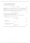
A.1 Scalar differential equations
Scalar ordinary differential equation of the form

dx
ẋ(t) = f (t, x(t)), ẋ(t) = (t) (A.1)
dt

Definition A.1: Let J ⊂ R be an interval. A function x : J → R is called a solution to the (scalar)
differential equation (in J) if x is differentiable, (t, x(t)) ∈ D for all t ∈ J, and (A.1) holds for all t ∈ J

Problem A.1: Initial value problem. Given a function f : D → R for some D ⊂ R × R and a point (t0 , x0 ),
find a solution x : J → R (as in Definition A.1 with J such that to ∈ J) such that

ẋ(t) = f (t, x(t)), x(t0 ) = x0 (A.6)

Here, the equation x(t0 ) = x0 is referred to as the initial condition.
x(·; t0 .x0 ) denotes a solution to the initial value problem.
Three classes of scalar differential equations for which solutions x can be computed explicitly:

• ẋ(t) = f (t)
where f is independent of x. The unique solution is given by
ˆ t
x(t) = x0 + f (τ ) dτ (A.10)
t0


• ẋ(t) = g(x(t))
The solution is given by
x(t) = ceat , c∈R (A.18)

• ẋ(t) = f (t)g(x(t)) (separable equations)
The solutions are given by: ˆ ˆ
1
dx = f (t)dt (A.25)
g(x)

Sometimes a solution does not exist for the entire domain, or it only exists as a piecewise function.




1

,A.2 Linear differential equations
A linear differential equation is of the form

ẋ(t) = a(t)x(t) + b(t) (A.37)

This is called homogeneous when b(t) = 0 and inhomogeneous otherwise.
The differential operator is L(x) = ẋ − a(t)x Homogeneous equations: ẋ(t) = a(t)x(t) which is separable and
has the class of solutions ˆ
x(t) = CeF (t) , F (t) = a(t) dt (A.44)

Lemma A.1 Consider the initial value problem ẋ(t) = a(t)x(t), x(t0 ) = x0 where a : J → R is continuous
and t0 ∈ J. Then, the unique solution for t ∈ J is
ˆ t
F (t)
x(t; t0 , x0 ) = x0 e , F (t) = a(τ )dτ (A.49)
t0


Nonhomogeneous equations
Lemma A.2 consider the initial value problem ẋ(t) = a(t)x(t) + b(t) , x(t0 ) = x0 where a, b : J → R are
continuous and t0 ∈ J. Then, for t ∈ J the unique solution is:
ˆ t ˆ t
x(t; t0 , x0 ) = x0 eF (t) + eF (t) e−F (τ ) b(τ )dτ , F (t) = a(τ )dτ (A.65)
t0 t0




2

, A.3 Systems of differential equations
A system of ODEs can be written as:

x˙1 (t) = f1 (t, x1 (t), . . . , xn (t))
..
. (A.79)
x˙n (t) = fn (t, x1 (t), . . . , xn (t))

We define: 
  
x1 f1 (t, x1 (t), . . . , xn (t))
 .   .. 
x= .  , f (t, x) =  (A.80)
 .  .

 
xn fn (t, x1 (t), . . . , xn (t))

So equation A.79 then becomes ẋ(t) = f (t, x(t))
√ p
Euclidean norm: |x| = xT x = x21 + x22 + · · · + x2n
Definition A.3 (Lipschitz continuity). A function f : D → Rn with D ⊂ R × Rn is called Lipschitz (in x)
at a point (t′ , x′ ) ∈ D if there exists constants L > 0 and r > 0 such that |f (t, x) − f (t, x′ )| ≤ L|x − x′ | for
all (t, x) such that |x − x′ | < r, |t − t′ | < r and (t, x) ∈ D. If f is Lipschitz (in x) for all (t′ , x′ ) ∈ D, it is
said to be locally Lipschitz (in x) on D.
Theorem A.3 Let f : D → Rn with domain D ⊂ R × Rn be continuous and locally Lipschitz (in x) on D.
If (t0 , x0 ) ∈ D, then there exists a solution to the initial value problem. This solution is unique and can be
extended to the left and right up to the boundary of D.
Any function that has infinite slope at some point is not Lipschitz at that point.
We can transform a higher order differential equation:

y (n) (t) = f (t, y(t), ẏ(t), . . . , y (n−1) (t)) (A.89)

By defining the following matrices:
h iT
T
x = [x1 x2 . . . xn ] = y ẏ . . . y (n−1)

Such that A.89 leads to:    
x˙1 (t) x2 (t)
   
 x˙2 (t)   x3 (t) 
.. ..
   
= (A.91)
   

 . 
 
 . 

xn−1
˙ (t)  xn (t)
   

x˙n (t) f (t, x1 , x2 , . . . , xn−2 (t), xn−1 (t))




3