Dynamic effects, market size; growth
If we are increasing the size of the economy, we get more firms sharing the market. This
requires these firms to enter in competition. All of a sudden, Dutch firms face competition
from Spanish firms. This encourages efficiencies. You get redistribution in a way that is more
efficient and you get an increase of output per worker.
A numerical example to get an idea:
Suppose you have three countries and ten car manufacturers.
• England 3
• France 3
• Germany 4
Before integration, English and French consumers could choose between 3 brands. Germans
could choose between 4. If you allow for integration to happen, instead of 10 manufacturers
in three different countries, you get 10 manufacturers in one big market. The bigger market
introducers bigger competition. This leads to a situation in which only some manufacturers
survive. In this case, four manufacturers leave the market because they don’t survive.
• England 0
• France 2
• Germany 4
The new situation provides more choices for consumers. The English had a choice of three
brands, they can now choose from six. The same goes for the French.
Time for an analysis of integration.
The left firm shows sales per firm and Euros. The average cost line (AC) is shown. At a
production of x’ the costs are equal to P’. With higher production, the costs will probably go
down. The middle graph shows the demand curve of the market. It shows more sales for
lower prices. If individual firms sell x’ at a price of P’, you get a total of C’ sales. You can see
this in the two graphs on the left. In this market you get a number of firms equal to n’.
n’ = C’/x’. Because the total firms are C’ and the sales per firm are x’.
The graph on the right is the most important one. It shows the number of firms and the
mark-up. We assume that the marginal costs (the cost of producing an additional unit of
output) is constant. Prices are marginal cost + mark-up. That is why the right-hand graph
, starts at the height of the marginal costs. If there is only one firm (monopoly), the mark-up
will be high. The more firms, the less options there are to increase mark-up. If the number of
firms increases, the mark-up is usually forced down. In the right-hand graph the competition
curve is shown. It is downwards sloping because the mark-up will likely be pushed down if
there are more firms. In the graph, the breakeven curve is also shown (BE). It shows the
number of firms that survive. With a high mark-up, a lot of firms can be allowed in the
market. The breakeven curve is upwards sloping. There is an equilibrium between these two
lines. Suppose you have a firm with a high mark-up. New firms join the market which leads
to a lower markup. As a result, the number of firms that survives drops. This will lead to an
equilibrium with a certain mark-up and number of firms at a certain price level.
This figure shows the merge of two identical countries. With two identical markets, the
m=home market can be supplied by twice as many firms. Because the two countries are
identical, you get 2n’ firms as shown in the righthand graph. This is because both countries
have n’ firms. At 2n’ we start in point 1, assuming that we are still at the same mark-up (u’).
At that point 2n’ number of firms should be able to survive. But, in reality, the mark-up will
be pushed down from u’ to uA. At uA 2n’ firms would not be able to survive. This means a
decrease of the number of firms to n’’. A new equilibrium is found at E’’. The price is then set
at P’’. Sales will go up to C’’ (but will drop from PA). For the firms that survive, sales go up to
x’’. The blue breakeven curve is the new breakeven curve with free trade (BEFT).
If we are increasing the size of the economy, we get more firms sharing the market. This
requires these firms to enter in competition. All of a sudden, Dutch firms face competition
from Spanish firms. This encourages efficiencies. You get redistribution in a way that is more
efficient and you get an increase of output per worker.
A numerical example to get an idea:
Suppose you have three countries and ten car manufacturers.
• England 3
• France 3
• Germany 4
Before integration, English and French consumers could choose between 3 brands. Germans
could choose between 4. If you allow for integration to happen, instead of 10 manufacturers
in three different countries, you get 10 manufacturers in one big market. The bigger market
introducers bigger competition. This leads to a situation in which only some manufacturers
survive. In this case, four manufacturers leave the market because they don’t survive.
• England 0
• France 2
• Germany 4
The new situation provides more choices for consumers. The English had a choice of three
brands, they can now choose from six. The same goes for the French.
Time for an analysis of integration.
The left firm shows sales per firm and Euros. The average cost line (AC) is shown. At a
production of x’ the costs are equal to P’. With higher production, the costs will probably go
down. The middle graph shows the demand curve of the market. It shows more sales for
lower prices. If individual firms sell x’ at a price of P’, you get a total of C’ sales. You can see
this in the two graphs on the left. In this market you get a number of firms equal to n’.
n’ = C’/x’. Because the total firms are C’ and the sales per firm are x’.
The graph on the right is the most important one. It shows the number of firms and the
mark-up. We assume that the marginal costs (the cost of producing an additional unit of
output) is constant. Prices are marginal cost + mark-up. That is why the right-hand graph
, starts at the height of the marginal costs. If there is only one firm (monopoly), the mark-up
will be high. The more firms, the less options there are to increase mark-up. If the number of
firms increases, the mark-up is usually forced down. In the right-hand graph the competition
curve is shown. It is downwards sloping because the mark-up will likely be pushed down if
there are more firms. In the graph, the breakeven curve is also shown (BE). It shows the
number of firms that survive. With a high mark-up, a lot of firms can be allowed in the
market. The breakeven curve is upwards sloping. There is an equilibrium between these two
lines. Suppose you have a firm with a high mark-up. New firms join the market which leads
to a lower markup. As a result, the number of firms that survives drops. This will lead to an
equilibrium with a certain mark-up and number of firms at a certain price level.
This figure shows the merge of two identical countries. With two identical markets, the
m=home market can be supplied by twice as many firms. Because the two countries are
identical, you get 2n’ firms as shown in the righthand graph. This is because both countries
have n’ firms. At 2n’ we start in point 1, assuming that we are still at the same mark-up (u’).
At that point 2n’ number of firms should be able to survive. But, in reality, the mark-up will
be pushed down from u’ to uA. At uA 2n’ firms would not be able to survive. This means a
decrease of the number of firms to n’’. A new equilibrium is found at E’’. The price is then set
at P’’. Sales will go up to C’’ (but will drop from PA). For the firms that survive, sales go up to
x’’. The blue breakeven curve is the new breakeven curve with free trade (BEFT).