1. Sample description
● Mean ӯ :
○ describes centrality, the average value
○ theoretically only for interval variables, but in practice used for ordinal
variables too
○ dichotomous variables → proportion
○ mean = sum of all values / number of observations
● Variance s2:
○ square of the standard deviation (s)
○ tells us how different people answer on one variable
○ measures dispersion in a variable
○ sum of all squared differences between observations and the mean, divided
by number of observation minus 1
● Standard deviation s
○ describes dispersion of data
○ summary measure of the average distance to the mean
■ if all observations are clustered around the mean, the sum of
distances will be small
■ if observations are widely dispersed around the mean, the sum of
distances will be larger
○ if there is more dispersion, the standard deviations will be higher.
○ square root of variance
○ square root of the sum of all differences between observations and the mean,
squared, divided by number of observation minus 1
● Covariance
○ the extent to which two variables vary with each other
■ e.g. if you score high on working hours, you score low on hours of
study, if you have many years of education, you often have a higher
income
○ when two variables (x and y) have a positive covariance: on average, those
that score high on x also score high on y
○ sum of all distances of an observation x to the mean of X (xi-x̅) multiplied by
the distance of an observation y to the mean of Y (yi-ӯ) divided by number of
observation minus one
, ○ covariance is difficult to interpret, standardized covariance → correlation
● Z-score
○ standardized measure of the distance to the mean.
○ number of standard deviations from the mean
○ z-scores take into account differences in both centrality and dispersion
○ z-scores help us to describe bell-shaped distributions
○ distance from the observation to the mean divided by standard deviation
2. Confidence intervals
● Confidence Interval for proportion
○ used for dichotomous variable
○ Proportion sample (πˆ)
○ Standard error for proportion (se)
○ Z-value - confidence level (Table A):
■ for 90% the z-value is 1.65
■ for 95% the z-value is 1.96.
■ for 99% the z-value is 2.58
● Standard error for proportion
○ standard error is the dispersion of the sampling distribution → how much
variation is there
○ standard error = square root of proportion multiplied by 1 minus the
proportion divided by sample size
● Confidence Interval for mean
○ used for interval or ordinal variable
○ Mean (ӯ)
○ Standard error (se)
○ Standard error for mean
○ T-value instead of z-value (Table B)
■ calculated based on degree of freedom (df): n-1
■ when the sample size is bigger than 100 the t-distribution follows the
z-distribution
● Standard error for mean
○ standard deviation divided by square root of sample size
● Mean ӯ :
○ describes centrality, the average value
○ theoretically only for interval variables, but in practice used for ordinal
variables too
○ dichotomous variables → proportion
○ mean = sum of all values / number of observations
● Variance s2:
○ square of the standard deviation (s)
○ tells us how different people answer on one variable
○ measures dispersion in a variable
○ sum of all squared differences between observations and the mean, divided
by number of observation minus 1
● Standard deviation s
○ describes dispersion of data
○ summary measure of the average distance to the mean
■ if all observations are clustered around the mean, the sum of
distances will be small
■ if observations are widely dispersed around the mean, the sum of
distances will be larger
○ if there is more dispersion, the standard deviations will be higher.
○ square root of variance
○ square root of the sum of all differences between observations and the mean,
squared, divided by number of observation minus 1
● Covariance
○ the extent to which two variables vary with each other
■ e.g. if you score high on working hours, you score low on hours of
study, if you have many years of education, you often have a higher
income
○ when two variables (x and y) have a positive covariance: on average, those
that score high on x also score high on y
○ sum of all distances of an observation x to the mean of X (xi-x̅) multiplied by
the distance of an observation y to the mean of Y (yi-ӯ) divided by number of
observation minus one
, ○ covariance is difficult to interpret, standardized covariance → correlation
● Z-score
○ standardized measure of the distance to the mean.
○ number of standard deviations from the mean
○ z-scores take into account differences in both centrality and dispersion
○ z-scores help us to describe bell-shaped distributions
○ distance from the observation to the mean divided by standard deviation
2. Confidence intervals
● Confidence Interval for proportion
○ used for dichotomous variable
○ Proportion sample (πˆ)
○ Standard error for proportion (se)
○ Z-value - confidence level (Table A):
■ for 90% the z-value is 1.65
■ for 95% the z-value is 1.96.
■ for 99% the z-value is 2.58
● Standard error for proportion
○ standard error is the dispersion of the sampling distribution → how much
variation is there
○ standard error = square root of proportion multiplied by 1 minus the
proportion divided by sample size
● Confidence Interval for mean
○ used for interval or ordinal variable
○ Mean (ӯ)
○ Standard error (se)
○ Standard error for mean
○ T-value instead of z-value (Table B)
■ calculated based on degree of freedom (df): n-1
■ when the sample size is bigger than 100 the t-distribution follows the
z-distribution
● Standard error for mean
○ standard deviation divided by square root of sample size