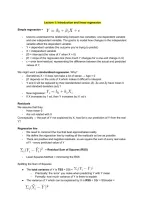
Lecture 1: Introduction and linear regression
Simple regression =
- Used to understand the relationship between two variables: one dependent variable
and one independent variable. The goal is to model how changes in the independent
variable affect the dependent variable.
- Y = dependent variable (the outcome you’re trying to predict)
- X = independent variable
- β0 = intercept (the value of Y when X = 0)
- β1= slope of the regression line (how much Y changes for a one-unit change in X)
- ϵ = error term/residual, representing the difference between the actual and predicted
values of Y.
We might want a standardized regression. Why?
- Sometimes X = 0 does not make a lot of sense → Age = 0
- β1depends on the units of X which makes it difficult to interpret
- Y and X will be replaced by their standardized version (Z). Zx and Zy have mean 0
and standard deviation (sd) 1
- New regression:
- If X increases by 1 sd, then Y increases by 𝑏1 sd’s
Residuals
We assume that they:
- Have mean 0
- Are not related with X
Conceptually → the part of Y not explained by X; how far is our prediction of Y from the real
Y?
Regression line
- We need to construct the line that best approximates reality
- We define the regression line by making all the residuals as low as possible
- There are positive and negative residuals, so we square the sum of every real value
of Y - every predicted value of Y
= Residual Sum of Squares (RSS)
- Least Squares Method = minimizing the RSS
Splitting the Sum of Squares
● The total variance of Y is TSS = SSt =
- Practically: the ‘error’ you make when predicting Y with Y mean
- Formally: how much variance of Y is there to explain
● The variance of Y which can be explained by X is RSS = SSr = SSmodel =
, - Practically: what the regression explains
● Finally, the variance of Y which cannot be explained by X is SSE = SSe =
- Practically: what the regression does not explain
Besides the totals, sometimes it is useful to see the mean errors
- To do this, we divide by the degrees of freedom
- Let’s say that k is the no. independent variables and N the sample, then:
Coefficient of determination R-squared
- R2 is the percentage (between 0 and 1) of the total variance that is explained by the
regression
- The percentage of unexplained variance is then: 1 - R2
Lecture 2: Multiple regression
Multiple regression = to explain Y as a function of several independent variables.
Example: explaining wage by education and age.
Causality
Question: is there a causal effect of X on Y?
Requirements for causality:
- X and Y are associated
- X (independent) is realized earlier than Y (dependent)
- We have excluded all other alternative explanations of Y
Keep in mind: correlation does not imply causation
We use multiple regression because we want to comply with the third requirement.
We exclude alternative explanations by controlling for several variables
- However, it is not that simple
We should think about controls in multiple regression falling within three cases or scenarios:
1. Not an alternative path: it might be the case that both X1 and X2 explain Y but they
do not relate to each other → X2 is a bad control
● Keep in mind that this is an extreme example; you rarely find this exact
situation
, 2. An alternative path: it could be that X2 does relate to X1, and thus it shows an
alternative path from X1 to Y.
● Usual suspects: fixed attributes (e.g., gender, age, country of origin)
3. Only one real path: on the other hand, if X1 and X2 are strongly related, the
coefficients might change considerably.
● If they are exactly the same, R would drop one since it’s completely
redundant.
● Adding variables that are too similar is also not desirable since it increases
the sd.
Regression interpretation
- For all coefficients the H0: 𝛽 = 0 is rejected (p < .001)
- 𝛽0 =−6.021 is the expected wage when 𝑎𝑔𝑒 = 0 and 𝑒𝑑𝑢𝑐𝑎𝑡𝑖𝑜𝑛 = 0
- 𝛽1 =0.901 expected increase of wage given an additional year of education, holding
constant the age
- 𝛽2 =0.257 expected increase of wage given an additional year of age, holding
constant the education
(ceteris paribus = everything else constant).
Since we keep all the remaining X constant, we call the 𝛽 effects partial regression
coefficients.
The questions we can answer with regression:
- What is the expected Y? → Find Y hat
- What is the effect (partial coefficient) of X on Y?
Recap on variance of Y
- R2: higher values imply that X predict Y quite well
Joint test
- Sometimes, we want to know if any (or a group) of our independent variables explain
Y → Nested models and F-test
- Nested models: a regression model with a subset of the X’s of another regression
● The unrestricted or full model has the larger number of variables
● The restricted or reduced model has the smaller number of variables
→ By comparing these two models we can talk about a joint test
Adjusted R2
● R2 in regression can be misleading
● The more variables (higher k) → higher the ESS → higher R2
● This does not necessarily mean that we are predicting better
→ To solve this problem, we can use the adjusted R2
● R2adj is usually smaller than R2 (R2adj can be 0, unlike the R2)