Summary Introduction to Statistical Analysis
Lecture week 1
Ways of classifying statistics:
Univariate One thing you are measuring (e.g. What was the average grade of the ISA exam last
year?)
Bivariate Relating one thing to another (e.g. Did males and females differ in their grades?). You
are relating gender to grades.
Multivariate Many different things and how they relate to one other thing (e.g. Was the grade
dependent on initial motivation, the time spent on reading and gender?)
Two types of different statistics:
Descriptive statistics Describing the pool of data that you have
Inferential statistics Taking numbers that are extracted, and drawing broader conclusions about
the population from them.
Unit of analysis The what or who that is being studied (e.g. individuals, groups, artifacts,
geographical units, social interactions, etc.)
Variable A measured property of the units of analysis
Levels of measurement
- Nominal (i.e. categorical levels) Group classifications, no measurement ranking possible.
- Ordinal Meaningful ranking, yet distance between categories is unknown or unequal.
- Interval Meaningful ranking, distance are equal (but no meaningful 0 point).
- Ratio Meaningful ranking, distances are equal (absolute and meaningful 0 point).
The ‘higher’ (interval/ratio) the level of measurement, the more ‘quantitative’ the variable is.
Continuous variables Measured along a continuum (e.g. temperature, grades, height, surface).
Numbers that have other numbers behind the comma (1.87 cm for height, 8.5 as a grade, etc.)
Note: Also averages! E.g. average number of children per woman in a country. You can have ‘2.3
children’.
Discrete variables Measured in whole units or categories (e.g. how many students are in this
room?) Whole numbers, thus: 126 students.
N = entire population
n = sample of population
Measures of central tendency To (univariate) describe the distribution of variables on different
levels of measurement. The measures of central tendency are the mean, median and mode.
1. The mean (M for sample, for population μ).
Mean All values are added up and divided by n, i.e. the number of observations in the sample.
,The Sum of Squares (SS) (the value 42 in this example)
A larger SS means that scores deviate more from the
mean. Squaring is done to correct for distances.
2. The median. How to find the median? 1. Sort all cases from lowest to highest. 2. The value of the
“middle case” equals the median (there is an equal amount of cases above and below this number).
In contrast to the mean, the median is not responsive to outliers.
Whenever n is an even number, the median is the mean value of the two middle cases.
3. The mode the category with the largest amount of cases.
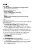
Normal and skewed distributions
Perfect normal distributions do not exist.
If the distributions leans to the right, it is left skewed (negatively skewed).
If the distributions leans to the left, it is rightly skewed (positively skewed).
The median is typically used to describe skewed distributions and ordinal scale data.
Week 1 - Book chapter 1 and chapter 3
Statistics is a branch of mathematics used to summarize, analyze, and interpret what we observe-to
make sense or meaning of our observations. Statistics is commonly applied to evaluate scientific
observations.
Mark Twain: There are lies, damned lies, and statistics. He meant that statistics could be deceiving,
and so can interpreting them.
In all, scales of measurement are characterized by three properties: order, difference, and ratio. Each
property can be described by answering the following questions:
1. Order: Does a larger number indicate a greater value than a smaller number?
2. Difference: Does subtracting two numbers represent some meaningful value?
3. Ratio: Does dividing (or taking the ratio of) two numbers represent some meaningful value?
Coding is the procedure of converting a nominal or categorical variable to a numeric value.
A true zero is when the value 0 truly indicates nothing on a scale of measurement. Interval scales do
not have a true zero (e.g. Celcius, Fahrenheit, pH).
,A quantitative variable varies by amount. This variable is measured numerically and is often
collected by measuring or counting.
A qualitative variable varies by class. This variable is often represented as a label and describes
nonnumeric aspects of phenomena.
A ratio scale variable can both be continuous or discrete. Qualitative variables can only be
discrete.
Chapter 3
Measures of central tendency are statistical measures for locating a single score that is most
representative or descriptive of all scores in a distribution (mean, median and mode). Measures of
central tendency are single values that have a "tendency" to be near the "center" of a distribution.
The difference of each score from the mean always sums to zero, similar to placing weights on both
sides of a scale. The mean would be located at the point that balances both ends the difference in
weight on each side would be zero.
Summing the squared differences of each score from its mean produces a minimal solution (i.e. the
smallest value). It is the smallest value for the sum of the squared differences of scores from their
mean. If you replace the mean with any other value, the solution will be larger.
The median is the midpoint in a distribution. Outliers in a data set influence the value of the mean,
but not the median. The 50th percentile of a cumulative percent distribution can be used to estimate
the value of the median (or look at Q2).
The normal distribution (also called the symmetrical, Gaussian, or bell-shaped distribution) is a
theoretical distribution in which scores are symmetrically distributed above and below the mean, the
median, and the mode at the center of the distribution.
A skewed distribution is a distribution of scores that includes outliers or scores that fall substantially
above or below most other scores in a data set.
A positively skewed distribution is a distribution of scores in which outliers are substantially
larger (toward the right tail in a graph) than most other scores.
A negatively skewed distribution is a distribution of scores in which outliers are substantially
smaller (toward the left tail in a graph) than most other scores.
,Types of distributions
A modal distribution is a distribution of scores in which one or more scores occur most often or most
frequently (there are also unimodal, bimodal, multimodal and nonmodal distributions, distributions
with one mode, two modes, more than two modes and no modes, respectively).
Standard normal distribution (name after z-transformation)
Normal distribution
Sample means distribution (used for one sample z-tests and t-tests, and confidence intervals)
Lecture week 2
Measures of variability
Another word for variability is dispersion. Measures of central tendency alone carry not enough
information to adequately describe distributions of variables, we need a second type of measures:
Measures of variability
- The range (ordinal, interval/ratio) the distance between the highest and lowest score.
The range is always reported together with maximum and minimum score. It is responsive/sensitive
to outliers.
- The interquartile range (IQR) (ordinal, interval/ratio) Based on ‘quartiles’ that split our data into
four equal groups of cases. You basically look for four medians.
The median quartile is Q2. For all four, you also look for Q1 and Q3. This gives you 4 different groups.
The interquartile range (IQR) is based on the distance between Q1 and Q3: IQR = Q3 – Q1.
What does this add to the range? Why might the IQR be a better measure?
The entire range include outliers, whereas the IQR captures the ‘middle section’ of the data which is
not sensitive to the outliers. It provides a better picture of scores.
- The variance Based on the sum of squares, i.e. the squared distance from the mean. For the
calculation of the variance, it matters whether we have sample data or population data (usually we
have sample data, but sometimes you have population data when the population is small enough).
An example of small population data could be ‘all your friends’. You might want to look at the
variance of the age of your friends.
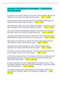
, An example of variance, calculated by hand:
How can we interpret the value of the variance? (e.g., 4.67) We don’t, but: “everything is
meaningful in comparison” (i.e. when comparing variances across groups, we can make comparative
statements about more/less dispersion around the mean).
For the purpose of interpretation, we calculate another measure of variability: the standard
deviation.
Why are there two different variance formulas for sample data / population data?
We often use the sample variance as an ‘estimator’ for the population variance (which is typically
unknown). When we calculate sample variance, we therefore divide by n-1, to arrive at an unbiased
estimator of the population variance. Note how this is particularly relevant in small samples.
Lecture week 1
Ways of classifying statistics:
Univariate One thing you are measuring (e.g. What was the average grade of the ISA exam last
year?)
Bivariate Relating one thing to another (e.g. Did males and females differ in their grades?). You
are relating gender to grades.
Multivariate Many different things and how they relate to one other thing (e.g. Was the grade
dependent on initial motivation, the time spent on reading and gender?)
Two types of different statistics:
Descriptive statistics Describing the pool of data that you have
Inferential statistics Taking numbers that are extracted, and drawing broader conclusions about
the population from them.
Unit of analysis The what or who that is being studied (e.g. individuals, groups, artifacts,
geographical units, social interactions, etc.)
Variable A measured property of the units of analysis
Levels of measurement
- Nominal (i.e. categorical levels) Group classifications, no measurement ranking possible.
- Ordinal Meaningful ranking, yet distance between categories is unknown or unequal.
- Interval Meaningful ranking, distance are equal (but no meaningful 0 point).
- Ratio Meaningful ranking, distances are equal (absolute and meaningful 0 point).
The ‘higher’ (interval/ratio) the level of measurement, the more ‘quantitative’ the variable is.
Continuous variables Measured along a continuum (e.g. temperature, grades, height, surface).
Numbers that have other numbers behind the comma (1.87 cm for height, 8.5 as a grade, etc.)
Note: Also averages! E.g. average number of children per woman in a country. You can have ‘2.3
children’.
Discrete variables Measured in whole units or categories (e.g. how many students are in this
room?) Whole numbers, thus: 126 students.
N = entire population
n = sample of population
Measures of central tendency To (univariate) describe the distribution of variables on different
levels of measurement. The measures of central tendency are the mean, median and mode.
1. The mean (M for sample, for population μ).
Mean All values are added up and divided by n, i.e. the number of observations in the sample.
,The Sum of Squares (SS) (the value 42 in this example)
A larger SS means that scores deviate more from the
mean. Squaring is done to correct for distances.
2. The median. How to find the median? 1. Sort all cases from lowest to highest. 2. The value of the
“middle case” equals the median (there is an equal amount of cases above and below this number).
In contrast to the mean, the median is not responsive to outliers.
Whenever n is an even number, the median is the mean value of the two middle cases.
3. The mode the category with the largest amount of cases.
Normal and skewed distributions
Perfect normal distributions do not exist.
If the distributions leans to the right, it is left skewed (negatively skewed).
If the distributions leans to the left, it is rightly skewed (positively skewed).
The median is typically used to describe skewed distributions and ordinal scale data.
Week 1 - Book chapter 1 and chapter 3
Statistics is a branch of mathematics used to summarize, analyze, and interpret what we observe-to
make sense or meaning of our observations. Statistics is commonly applied to evaluate scientific
observations.
Mark Twain: There are lies, damned lies, and statistics. He meant that statistics could be deceiving,
and so can interpreting them.
In all, scales of measurement are characterized by three properties: order, difference, and ratio. Each
property can be described by answering the following questions:
1. Order: Does a larger number indicate a greater value than a smaller number?
2. Difference: Does subtracting two numbers represent some meaningful value?
3. Ratio: Does dividing (or taking the ratio of) two numbers represent some meaningful value?
Coding is the procedure of converting a nominal or categorical variable to a numeric value.
A true zero is when the value 0 truly indicates nothing on a scale of measurement. Interval scales do
not have a true zero (e.g. Celcius, Fahrenheit, pH).
,A quantitative variable varies by amount. This variable is measured numerically and is often
collected by measuring or counting.
A qualitative variable varies by class. This variable is often represented as a label and describes
nonnumeric aspects of phenomena.
A ratio scale variable can both be continuous or discrete. Qualitative variables can only be
discrete.
Chapter 3
Measures of central tendency are statistical measures for locating a single score that is most
representative or descriptive of all scores in a distribution (mean, median and mode). Measures of
central tendency are single values that have a "tendency" to be near the "center" of a distribution.
The difference of each score from the mean always sums to zero, similar to placing weights on both
sides of a scale. The mean would be located at the point that balances both ends the difference in
weight on each side would be zero.
Summing the squared differences of each score from its mean produces a minimal solution (i.e. the
smallest value). It is the smallest value for the sum of the squared differences of scores from their
mean. If you replace the mean with any other value, the solution will be larger.
The median is the midpoint in a distribution. Outliers in a data set influence the value of the mean,
but not the median. The 50th percentile of a cumulative percent distribution can be used to estimate
the value of the median (or look at Q2).
The normal distribution (also called the symmetrical, Gaussian, or bell-shaped distribution) is a
theoretical distribution in which scores are symmetrically distributed above and below the mean, the
median, and the mode at the center of the distribution.
A skewed distribution is a distribution of scores that includes outliers or scores that fall substantially
above or below most other scores in a data set.
A positively skewed distribution is a distribution of scores in which outliers are substantially
larger (toward the right tail in a graph) than most other scores.
A negatively skewed distribution is a distribution of scores in which outliers are substantially
smaller (toward the left tail in a graph) than most other scores.
,Types of distributions
A modal distribution is a distribution of scores in which one or more scores occur most often or most
frequently (there are also unimodal, bimodal, multimodal and nonmodal distributions, distributions
with one mode, two modes, more than two modes and no modes, respectively).
Standard normal distribution (name after z-transformation)
Normal distribution
Sample means distribution (used for one sample z-tests and t-tests, and confidence intervals)
Lecture week 2
Measures of variability
Another word for variability is dispersion. Measures of central tendency alone carry not enough
information to adequately describe distributions of variables, we need a second type of measures:
Measures of variability
- The range (ordinal, interval/ratio) the distance between the highest and lowest score.
The range is always reported together with maximum and minimum score. It is responsive/sensitive
to outliers.
- The interquartile range (IQR) (ordinal, interval/ratio) Based on ‘quartiles’ that split our data into
four equal groups of cases. You basically look for four medians.
The median quartile is Q2. For all four, you also look for Q1 and Q3. This gives you 4 different groups.
The interquartile range (IQR) is based on the distance between Q1 and Q3: IQR = Q3 – Q1.
What does this add to the range? Why might the IQR be a better measure?
The entire range include outliers, whereas the IQR captures the ‘middle section’ of the data which is
not sensitive to the outliers. It provides a better picture of scores.
- The variance Based on the sum of squares, i.e. the squared distance from the mean. For the
calculation of the variance, it matters whether we have sample data or population data (usually we
have sample data, but sometimes you have population data when the population is small enough).
An example of small population data could be ‘all your friends’. You might want to look at the
variance of the age of your friends.
, An example of variance, calculated by hand:
How can we interpret the value of the variance? (e.g., 4.67) We don’t, but: “everything is
meaningful in comparison” (i.e. when comparing variances across groups, we can make comparative
statements about more/less dispersion around the mean).
For the purpose of interpretation, we calculate another measure of variability: the standard
deviation.
Why are there two different variance formulas for sample data / population data?
We often use the sample variance as an ‘estimator’ for the population variance (which is typically
unknown). When we calculate sample variance, we therefore divide by n-1, to arrive at an unbiased
estimator of the population variance. Note how this is particularly relevant in small samples.