PRACTICAL EXERCISE 12: SOLUTION
1. Start a log file in your folder (call it model select.log)
2. Open the dataset model select 1.dta.
3. The dataset gives data on the real gross domestic product (y), labour input (x2), and real capital input
(x3) in the manufacturing sector for a developing country for the years 1958 to 1972. Suppose that the
theoretically correct production function is of the Cobb-Douglas type. Our model can be specified as
follows:
ln Y t B ln
= B1 + 2
X2 t +
B 3 ln X 3 t u
+ t
Where ln = the natural log.
4. Generate logged values of y, x2 and x3. Type:
gen lnY = log(y)
gen lnX2=log(x2)
gen lnX3=log(x3)
5. Using regression, estimate the Cobb-Douglas production function for this country for the sample
period and interpret the results.
reg lnY lnX2 lnX3
Source | SS df MS Number of obs = 15
-------------+------------------------------ F( 2, 12) = 362.36
Model | 4.41639958 2 2.20819979 Prob > F = 0.0000
Residual | .073127514 12 .006093959 R-squared = 0.9837
-------------+------------------------------ Adj R-squared = 0.9810
Total | 4.4895271 14 .320680507 Root MSE = .07806
------------------------------------------------------------------------------
lnY | Coef. Std. Err. t P>|t| [95% Conf. Interval]
-------------+----------------------------------------------------------------
lnX2 | .7147795 .1532679 4.66 0.001 .3808375 1.048722
lnX3 | 1.113473 .2991549 3.72 0.003 .4616705 1.765276
_cons | -7.843845 2.67984 -2.93 0.013 -13.68271 -2.004975
------------------------------------------------------------------------------
Based on the above results,
Coefficient of lnX2: keeping capital constant, the output-labour elasticity is 0.7148, on
average. OR ceteris paribus, a 1% increase in the labour input results in 0.7148% increase
in output, on average.
Coefficient of lnX3: keeping labour constant, the output-capital elasticity is 1.1135, on
average. OR ceteris paribus, a 1% increase in the capital input results in 1.1135%
increase in output, on average.
Both coefficients are individually statistically significant at all conventional levels.
Prac 12 – Model Selection – Solution Page 1 of 10
, 6. Now suppose that capital data (i.e. X3) were not initially available and therefore you estimated the
following production function:
ln Y t =A 1 + A 2 X 2t +v t
v
where t = error term.
Run the above regression and examine the consequences. What difference(s) do you note with regard
to the estimated coefficient values (i.e. elasticity values), the standard errors and the R2 values?
. reg lnY lnX2
Source | SS df MS Number of obs = 15
-------------+------------------------------ F( 1, 13) = 357.44
Model | 4.33197542 1 4.33197542 Prob > F = 0.0000
Residual | .157551678 13 .01211936 R-squared = 0.9649
-------------+------------------------------ Adj R-squared = 0.9622
Total | 4.4895271 14 .320680507 Root MSE = .11009
------------------------------------------------------------------------------
lnY | Coef. Std. Err. t P>|t| [95% Conf. Interval]
-------------+----------------------------------------------------------------
lnX2 | 1.257567 .0665163 18.91 0.000 1.113867 1.401267
_cons | 2.069561 .4177431 4.95 0.000 1.167082 2.97204
Since we have excluded the capital input variable from this model, the estimated
output-labor elasticity of 1.2576 is a biased estimate of the true elasticity. In the
true model (in 5 above), this estimate was 0.7148, which is much smaller than
1.2576. Even the R2 value in the misspecified model is somewhat smaller than the
‘correctly’ specified model, which was to be expected since we had excluded a
relevant variable from the former.
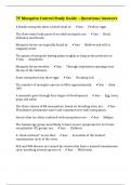
7. To estimate the extent of the bias in the above regression and assess whether it is upward or
downward, regress
ln X 3 on ln X 2 (refer to “Note on Omitted Variable Bias”).
. reg lnX3 lnX2
Source | SS df MS Number of obs = 15
-------------+------------------------------ F( 1, 13) = 124.27
Model | .650914498 1 .650914498 Prob > F = 0.0000
Residual | .068093767 13 .005237982 R-squared = 0.9053
-------------+------------------------------ Adj R-squared = 0.8980
Total | .719008265 14 .051357733 Root MSE = .07237
------------------------------------------------------------------------------
lnX3 | Coef. Std. Err. t P>|t| [95% Conf. Interval]
-------------+----------------------------------------------------------------
lnX2 | .4874725 .0437291 11.15 0.000 .3930016 .5819433
_cons | 8.903139 .2746322 32.42 0.000 8.309833 9.496446
------------------------------------------------------------------------------
Prac 12 – Model Selection – Solution Page 2 of 10
1. Start a log file in your folder (call it model select.log)
2. Open the dataset model select 1.dta.
3. The dataset gives data on the real gross domestic product (y), labour input (x2), and real capital input
(x3) in the manufacturing sector for a developing country for the years 1958 to 1972. Suppose that the
theoretically correct production function is of the Cobb-Douglas type. Our model can be specified as
follows:
ln Y t B ln
= B1 + 2
X2 t +
B 3 ln X 3 t u
+ t
Where ln = the natural log.
4. Generate logged values of y, x2 and x3. Type:
gen lnY = log(y)
gen lnX2=log(x2)
gen lnX3=log(x3)
5. Using regression, estimate the Cobb-Douglas production function for this country for the sample
period and interpret the results.
reg lnY lnX2 lnX3
Source | SS df MS Number of obs = 15
-------------+------------------------------ F( 2, 12) = 362.36
Model | 4.41639958 2 2.20819979 Prob > F = 0.0000
Residual | .073127514 12 .006093959 R-squared = 0.9837
-------------+------------------------------ Adj R-squared = 0.9810
Total | 4.4895271 14 .320680507 Root MSE = .07806
------------------------------------------------------------------------------
lnY | Coef. Std. Err. t P>|t| [95% Conf. Interval]
-------------+----------------------------------------------------------------
lnX2 | .7147795 .1532679 4.66 0.001 .3808375 1.048722
lnX3 | 1.113473 .2991549 3.72 0.003 .4616705 1.765276
_cons | -7.843845 2.67984 -2.93 0.013 -13.68271 -2.004975
------------------------------------------------------------------------------
Based on the above results,
Coefficient of lnX2: keeping capital constant, the output-labour elasticity is 0.7148, on
average. OR ceteris paribus, a 1% increase in the labour input results in 0.7148% increase
in output, on average.
Coefficient of lnX3: keeping labour constant, the output-capital elasticity is 1.1135, on
average. OR ceteris paribus, a 1% increase in the capital input results in 1.1135%
increase in output, on average.
Both coefficients are individually statistically significant at all conventional levels.
Prac 12 – Model Selection – Solution Page 1 of 10
, 6. Now suppose that capital data (i.e. X3) were not initially available and therefore you estimated the
following production function:
ln Y t =A 1 + A 2 X 2t +v t
v
where t = error term.
Run the above regression and examine the consequences. What difference(s) do you note with regard
to the estimated coefficient values (i.e. elasticity values), the standard errors and the R2 values?
. reg lnY lnX2
Source | SS df MS Number of obs = 15
-------------+------------------------------ F( 1, 13) = 357.44
Model | 4.33197542 1 4.33197542 Prob > F = 0.0000
Residual | .157551678 13 .01211936 R-squared = 0.9649
-------------+------------------------------ Adj R-squared = 0.9622
Total | 4.4895271 14 .320680507 Root MSE = .11009
------------------------------------------------------------------------------
lnY | Coef. Std. Err. t P>|t| [95% Conf. Interval]
-------------+----------------------------------------------------------------
lnX2 | 1.257567 .0665163 18.91 0.000 1.113867 1.401267
_cons | 2.069561 .4177431 4.95 0.000 1.167082 2.97204
Since we have excluded the capital input variable from this model, the estimated
output-labor elasticity of 1.2576 is a biased estimate of the true elasticity. In the
true model (in 5 above), this estimate was 0.7148, which is much smaller than
1.2576. Even the R2 value in the misspecified model is somewhat smaller than the
‘correctly’ specified model, which was to be expected since we had excluded a
relevant variable from the former.
7. To estimate the extent of the bias in the above regression and assess whether it is upward or
downward, regress
ln X 3 on ln X 2 (refer to “Note on Omitted Variable Bias”).
. reg lnX3 lnX2
Source | SS df MS Number of obs = 15
-------------+------------------------------ F( 1, 13) = 124.27
Model | .650914498 1 .650914498 Prob > F = 0.0000
Residual | .068093767 13 .005237982 R-squared = 0.9053
-------------+------------------------------ Adj R-squared = 0.8980
Total | .719008265 14 .051357733 Root MSE = .07237
------------------------------------------------------------------------------
lnX3 | Coef. Std. Err. t P>|t| [95% Conf. Interval]
-------------+----------------------------------------------------------------
lnX2 | .4874725 .0437291 11.15 0.000 .3930016 .5819433
_cons | 8.903139 .2746322 32.42 0.000 8.309833 9.496446
------------------------------------------------------------------------------
Prac 12 – Model Selection – Solution Page 2 of 10