Probability Theory – explained from scratch (L1–10) ESE EUR, FEB21005X · Levi S., MSc
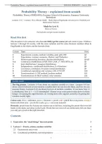
Probability Theory – explained from scratch
Probability Theory (FEB21005X), Erasmus School of Economics, Erasmus University
Rotterdam
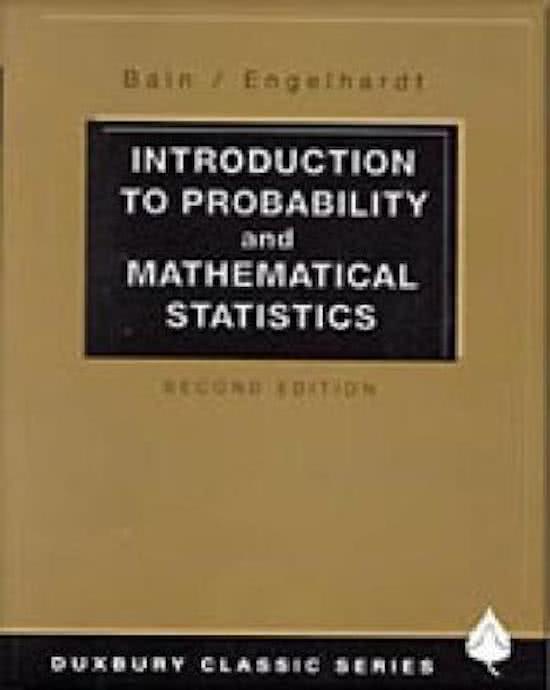
Lectures 1–10 · Lecturer: Dr. ir. Sharon Schalk · Book: Bain & Engelhardt, Introduction to Probability and
Mathematical Statistics
Made by Levi S.
Master of Science
For bachelor and pre-master students
Read this first
This document is for someone who does not (fully) get the course yet and wants to pass. It follows
lectures 1 through 10 exactly, with the same notation and the same theorem numbers (Bain &
Engelhardt) as the slides and the formula sheet.
Lecture Topic Here
1 Experiments, axioms, random variables, pmf, pdf, CDF §2
2 Expectation, variance, moments, Markov and Chebyshev §3
3 Moment generating functions, discrete distributions §4–§5
3–4 Continuous distributions (UNIF, EXP, GAM, χ2 , WEI, BETA, N) §6
5 Joint distributions I, marginal distributions §7
6 Independence, conditional distributions, E of functions §8
7 Covariance, correlation, bivariate normal distribution §9
8 Conditional expectation and variance, LTE, CVF, LTP §10
9 Transformations I: CDF method, Jacobian method §11
10 Transformations II: MGF method, order statistics §12
In plain words
The big picture. Lectures 1–4 are about one random variable at a time. Lectures 5–8 are
about relations between several random variables (how do you describe them, and how do you
measure them). Lectures 9–10 are about functions of random variables: if you know how X
is distributed, how is Y = h( X ) distributed? Almost every exam point comes down to three
things: (1) naming the right theorem, (2) writing down the support correctly, (3) getting the
notation exactly right.
Colour code. Blue = definition, green = theorem (+ proof), red = pitfall that costs points, orange =
homework (hint only – you do the work), grey = not exam material.
Honestly: proofs from the lectures are written out in full here, including the proofs that were left
blank on the slides and done on the board. Proofs that are homework are deliberately left out; there
you only get a push in the right direction.
Contents
1 Exam rules: the “small things” that cost points 3
2 Lecture 1 – Events, axioms, random variables 4
2.1 Experiments and events . . . . . . . . . . . . . . . . . . . . . . . . . . . . . . . . . . . 4
2.2 Conditional probability and independence . . . . . . . . . . . . . . . . . . . . . . . . 4
1
,Probability Theory – explained from scratch (L1–10) ESE EUR, FEB21005X · Levi S., MSc
2.3 Random variables, pmf, support . . . . . . . . . . . . . . . . . . . . . . . . . . . . . . 4
2.4 Cumulative distribution function . . . . . . . . . . . . . . . . . . . . . . . . . . . . . . 5
2.5 Continuous random variables and pdf . . . . . . . . . . . . . . . . . . . . . . . . . . . 5
3 Lecture 2 – Expectation, variance, moments, inequalities 6
4 Lecture 3a – Moment generating functions 7
5 Lecture 3b – Discrete distributions 8
6 Lectures 3c–4 – Continuous distributions 9
6.1 Uniform . . . . . . . . . . . . . . . . . . . . . . . . . . . . . . . . . . . . . . . . . . . . 9
6.2 Exponential . . . . . . . . . . . . . . . . . . . . . . . . . . . . . . . . . . . . . . . . . . 9
6.3 Gamma function, Gamma, χ2 , Weibull, Beta . . . . . . . . . . . . . . . . . . . . . . . . 10
6.4 Normal . . . . . . . . . . . . . . . . . . . . . . . . . . . . . . . . . . . . . . . . . . . . . 10
7 Lecture 5 – Joint distributions I 11
8 Lecture 6 – Independence, conditional distributions 12
9 Lecture 7 – Covariance, correlation, bivariate normal distribution 14
9.1 Covariance . . . . . . . . . . . . . . . . . . . . . . . . . . . . . . . . . . . . . . . . . . . 14
9.2 Variance of a linear combination . . . . . . . . . . . . . . . . . . . . . . . . . . . . . . 15
9.3 Correlation coefficient . . . . . . . . . . . . . . . . . . . . . . . . . . . . . . . . . . . . 15
9.4 Bivariate normal distribution . . . . . . . . . . . . . . . . . . . . . . . . . . . . . . . . 16
10 Lecture 8 – Conditional expectation and variance 17
10.1 Conditioning on an event . . . . . . . . . . . . . . . . . . . . . . . . . . . . . . . . . . 17
10.2 Conditioning on a random variable and the LTE . . . . . . . . . . . . . . . . . . . . . 18
10.3 Conditional variance and the CVF . . . . . . . . . . . . . . . . . . . . . . . . . . . . . 19
10.4 Conditional probability and the LTP . . . . . . . . . . . . . . . . . . . . . . . . . . . . 20
11 Lecture 9 – Transformations I 21
11.1 Univariate CDF method . . . . . . . . . . . . . . . . . . . . . . . . . . . . . . . . . . . 21
11.2 Bivariate CDF method . . . . . . . . . . . . . . . . . . . . . . . . . . . . . . . . . . . . 21
11.3 Univariate Jacobian method . . . . . . . . . . . . . . . . . . . . . . . . . . . . . . . . . 22
11.4 Multivariate Jacobian method . . . . . . . . . . . . . . . . . . . . . . . . . . . . . . . . 23
12 Lecture 10 – Transformations II: MGF method and order statistics 24
12.1 The MGF method . . . . . . . . . . . . . . . . . . . . . . . . . . . . . . . . . . . . . . . 24
12.2 Samples and order statistics . . . . . . . . . . . . . . . . . . . . . . . . . . . . . . . . . 25
13 Which method do I choose? (transformations) 27
14 Toolbox: tricks that recur everywhere 27
2
, Probability Theory – explained from scratch (L1–10) ESE EUR, FEB21005X · Levi S., MSc
15 Inconsistencies in the course material (be aware!) 28
16 Checklist before you hand in an answer 28
1 Exam rules: the “small things” that cost points
From the official exam information – memorise this
• A derived pdf or CDF must be defined for all x ∈ R: always write “0 otherwise” (for a
CDF: 0 to the left, 1 to the right).
• Introduce every random variable in words before you start calculating (“Let X denote the
number of . . . ”).
• If you use independence in a step, say so explicitly.
• Write X ∼ UNIF( a, b), never X = UNIF( a, b).
• Write ≈ (not =) after rounding or after using a table.
• Independence via f ( x, y) = f X ( x ) · f Y (y) requires the phrase “for all x, y ∈ R”.
• Write X | (Y = y). The notation X | Y has no meaning in this course.
R∞
• E( X ) = −∞ 12 dx for X ∼ UNIF(0, 2) is wrong twice: the integrand must be x · f X ( x ), and
R∞ R2
f X is 0 outside (0, 2). Correct: E( X ) = −∞ x · f X ( x ) dx = 0 x · 12 dx = 1.
• If the support of a joint pdf is a Cartesian product, you cannot use Theorem 4.4.2 to prove
dependence.
• Lecture 8: clearly show the switch from conditioning on an event to conditioning on a
random variable, and put LTE / CVF / LTP above the = sign.
• Lecture 9: with the Jacobian method for 2 variables, write down the general formula and
clearly indicate the inverse transformation, the Jacobian, the new pdf and its support.
• Applying LTE, CVF or LTP to objects that are not random variables costs points.
• Results from Examples 10.2, 10.4, 10.5, 10.6 may be used without proof, unless the question
says “use the MGF method to prove/show/derive. . . ”; then add a proof like the one of
Example 10.2.
Theorems you must state in full before using them (L1–10): Theorems 2.2.1, 2.3.1, 4.2.1, 4.3.1
(defining properties), Markov, Chebyshev, Theorem 4.4.1a (say which statement you use), Theorem
4.4.2. (Later: Law of Large Numbers and Central Limit Theorem, lecture 11.)
R∞
Formulas that earn points (write them down before applying them): E( X ) = −∞ x · f X ( x ) dx,
R∞
E( X 2 ) = −∞ x2 · f X ( x ) dx, E(h( X, Y )) = h( x, y) · f X,Y ( x, y) dx dy, µ′k = E( X k ), µk = E(( X −
RR
Cov( X, Y )
µ)k ), Var( X ) = E( X 2 ) − (E( X ))2 , Cov( X, Y ) = E( X · Y ) − E( X ) · E(Y ), ρ X,Y = ,
σX · σY
covariance matrix Σ, marginal pdf, conditional pdf, E( X | Y = y), both Jacobian formulas, LTE,
CVF, LTP.
Not exam material (L1–10): proofs of Markov and Chebyshev; proofs of the properties of the
Gamma function; proof that Xi ∼ BIN(n, pi ) in the multinomial for k = 3; derivation of the Law
of Total Probability; derivation of the covariance of the multinomial distribution; slides 9.26–9.27
(Jacobian method when h is not invertible).
g(k) ( a )
Memorise: Markov, Chebyshev, Taylor series g( x ) = ∑∞ k =0
k
k! ( x − a ) , the joint pdf and the
marginal pdf of the i-th order statistic Yi:n . (Later: CLT, convergence definitions.) You do not need to
memorise the pdf of the bivariate normal distribution.
3
Probability Theory – explained from scratch
Probability Theory (FEB21005X), Erasmus School of Economics, Erasmus University
Rotterdam
Lectures 1–10 · Lecturer: Dr. ir. Sharon Schalk · Book: Bain & Engelhardt, Introduction to Probability and
Mathematical Statistics
Made by Levi S.
Master of Science
For bachelor and pre-master students
Read this first
This document is for someone who does not (fully) get the course yet and wants to pass. It follows
lectures 1 through 10 exactly, with the same notation and the same theorem numbers (Bain &
Engelhardt) as the slides and the formula sheet.
Lecture Topic Here
1 Experiments, axioms, random variables, pmf, pdf, CDF §2
2 Expectation, variance, moments, Markov and Chebyshev §3
3 Moment generating functions, discrete distributions §4–§5
3–4 Continuous distributions (UNIF, EXP, GAM, χ2 , WEI, BETA, N) §6
5 Joint distributions I, marginal distributions §7
6 Independence, conditional distributions, E of functions §8
7 Covariance, correlation, bivariate normal distribution §9
8 Conditional expectation and variance, LTE, CVF, LTP §10
9 Transformations I: CDF method, Jacobian method §11
10 Transformations II: MGF method, order statistics §12
In plain words
The big picture. Lectures 1–4 are about one random variable at a time. Lectures 5–8 are
about relations between several random variables (how do you describe them, and how do you
measure them). Lectures 9–10 are about functions of random variables: if you know how X
is distributed, how is Y = h( X ) distributed? Almost every exam point comes down to three
things: (1) naming the right theorem, (2) writing down the support correctly, (3) getting the
notation exactly right.
Colour code. Blue = definition, green = theorem (+ proof), red = pitfall that costs points, orange =
homework (hint only – you do the work), grey = not exam material.
Honestly: proofs from the lectures are written out in full here, including the proofs that were left
blank on the slides and done on the board. Proofs that are homework are deliberately left out; there
you only get a push in the right direction.
Contents
1 Exam rules: the “small things” that cost points 3
2 Lecture 1 – Events, axioms, random variables 4
2.1 Experiments and events . . . . . . . . . . . . . . . . . . . . . . . . . . . . . . . . . . . 4
2.2 Conditional probability and independence . . . . . . . . . . . . . . . . . . . . . . . . 4
1
,Probability Theory – explained from scratch (L1–10) ESE EUR, FEB21005X · Levi S., MSc
2.3 Random variables, pmf, support . . . . . . . . . . . . . . . . . . . . . . . . . . . . . . 4
2.4 Cumulative distribution function . . . . . . . . . . . . . . . . . . . . . . . . . . . . . . 5
2.5 Continuous random variables and pdf . . . . . . . . . . . . . . . . . . . . . . . . . . . 5
3 Lecture 2 – Expectation, variance, moments, inequalities 6
4 Lecture 3a – Moment generating functions 7
5 Lecture 3b – Discrete distributions 8
6 Lectures 3c–4 – Continuous distributions 9
6.1 Uniform . . . . . . . . . . . . . . . . . . . . . . . . . . . . . . . . . . . . . . . . . . . . 9
6.2 Exponential . . . . . . . . . . . . . . . . . . . . . . . . . . . . . . . . . . . . . . . . . . 9
6.3 Gamma function, Gamma, χ2 , Weibull, Beta . . . . . . . . . . . . . . . . . . . . . . . . 10
6.4 Normal . . . . . . . . . . . . . . . . . . . . . . . . . . . . . . . . . . . . . . . . . . . . . 10
7 Lecture 5 – Joint distributions I 11
8 Lecture 6 – Independence, conditional distributions 12
9 Lecture 7 – Covariance, correlation, bivariate normal distribution 14
9.1 Covariance . . . . . . . . . . . . . . . . . . . . . . . . . . . . . . . . . . . . . . . . . . . 14
9.2 Variance of a linear combination . . . . . . . . . . . . . . . . . . . . . . . . . . . . . . 15
9.3 Correlation coefficient . . . . . . . . . . . . . . . . . . . . . . . . . . . . . . . . . . . . 15
9.4 Bivariate normal distribution . . . . . . . . . . . . . . . . . . . . . . . . . . . . . . . . 16
10 Lecture 8 – Conditional expectation and variance 17
10.1 Conditioning on an event . . . . . . . . . . . . . . . . . . . . . . . . . . . . . . . . . . 17
10.2 Conditioning on a random variable and the LTE . . . . . . . . . . . . . . . . . . . . . 18
10.3 Conditional variance and the CVF . . . . . . . . . . . . . . . . . . . . . . . . . . . . . 19
10.4 Conditional probability and the LTP . . . . . . . . . . . . . . . . . . . . . . . . . . . . 20
11 Lecture 9 – Transformations I 21
11.1 Univariate CDF method . . . . . . . . . . . . . . . . . . . . . . . . . . . . . . . . . . . 21
11.2 Bivariate CDF method . . . . . . . . . . . . . . . . . . . . . . . . . . . . . . . . . . . . 21
11.3 Univariate Jacobian method . . . . . . . . . . . . . . . . . . . . . . . . . . . . . . . . . 22
11.4 Multivariate Jacobian method . . . . . . . . . . . . . . . . . . . . . . . . . . . . . . . . 23
12 Lecture 10 – Transformations II: MGF method and order statistics 24
12.1 The MGF method . . . . . . . . . . . . . . . . . . . . . . . . . . . . . . . . . . . . . . . 24
12.2 Samples and order statistics . . . . . . . . . . . . . . . . . . . . . . . . . . . . . . . . . 25
13 Which method do I choose? (transformations) 27
14 Toolbox: tricks that recur everywhere 27
2
, Probability Theory – explained from scratch (L1–10) ESE EUR, FEB21005X · Levi S., MSc
15 Inconsistencies in the course material (be aware!) 28
16 Checklist before you hand in an answer 28
1 Exam rules: the “small things” that cost points
From the official exam information – memorise this
• A derived pdf or CDF must be defined for all x ∈ R: always write “0 otherwise” (for a
CDF: 0 to the left, 1 to the right).
• Introduce every random variable in words before you start calculating (“Let X denote the
number of . . . ”).
• If you use independence in a step, say so explicitly.
• Write X ∼ UNIF( a, b), never X = UNIF( a, b).
• Write ≈ (not =) after rounding or after using a table.
• Independence via f ( x, y) = f X ( x ) · f Y (y) requires the phrase “for all x, y ∈ R”.
• Write X | (Y = y). The notation X | Y has no meaning in this course.
R∞
• E( X ) = −∞ 12 dx for X ∼ UNIF(0, 2) is wrong twice: the integrand must be x · f X ( x ), and
R∞ R2
f X is 0 outside (0, 2). Correct: E( X ) = −∞ x · f X ( x ) dx = 0 x · 12 dx = 1.
• If the support of a joint pdf is a Cartesian product, you cannot use Theorem 4.4.2 to prove
dependence.
• Lecture 8: clearly show the switch from conditioning on an event to conditioning on a
random variable, and put LTE / CVF / LTP above the = sign.
• Lecture 9: with the Jacobian method for 2 variables, write down the general formula and
clearly indicate the inverse transformation, the Jacobian, the new pdf and its support.
• Applying LTE, CVF or LTP to objects that are not random variables costs points.
• Results from Examples 10.2, 10.4, 10.5, 10.6 may be used without proof, unless the question
says “use the MGF method to prove/show/derive. . . ”; then add a proof like the one of
Example 10.2.
Theorems you must state in full before using them (L1–10): Theorems 2.2.1, 2.3.1, 4.2.1, 4.3.1
(defining properties), Markov, Chebyshev, Theorem 4.4.1a (say which statement you use), Theorem
4.4.2. (Later: Law of Large Numbers and Central Limit Theorem, lecture 11.)
R∞
Formulas that earn points (write them down before applying them): E( X ) = −∞ x · f X ( x ) dx,
R∞
E( X 2 ) = −∞ x2 · f X ( x ) dx, E(h( X, Y )) = h( x, y) · f X,Y ( x, y) dx dy, µ′k = E( X k ), µk = E(( X −
RR
Cov( X, Y )
µ)k ), Var( X ) = E( X 2 ) − (E( X ))2 , Cov( X, Y ) = E( X · Y ) − E( X ) · E(Y ), ρ X,Y = ,
σX · σY
covariance matrix Σ, marginal pdf, conditional pdf, E( X | Y = y), both Jacobian formulas, LTE,
CVF, LTP.
Not exam material (L1–10): proofs of Markov and Chebyshev; proofs of the properties of the
Gamma function; proof that Xi ∼ BIN(n, pi ) in the multinomial for k = 3; derivation of the Law
of Total Probability; derivation of the covariance of the multinomial distribution; slides 9.26–9.27
(Jacobian method when h is not invertible).
g(k) ( a )
Memorise: Markov, Chebyshev, Taylor series g( x ) = ∑∞ k =0
k
k! ( x − a ) , the joint pdf and the
marginal pdf of the i-th order statistic Yi:n . (Later: CLT, convergence definitions.) You do not need to
memorise the pdf of the bivariate normal distribution.
3