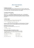
Matrix Analysis Optimization
Chapter 12
12.1 Matrices and vectors
A matrix has m rows and n columns. A matrix with only one row or column is called a vector.
If m = n, so that it has the same number of columns as rows, it’s called a square matrix of order
n. In this case, A= (aij)n×n. Only square matrices have a main diagonal.
12.2 Systems of linear equations
Here a11, a12,..., amn are called the coefficients of the system, and b1,...,bm are called the
constant terms, or right-hand sides. All of them are real numbers. If the above system has at
least one solution, it is said to be consistent. When the system has no solution, it is said to be
inconsistent.
12.3 Matrix Addition
We add two matrices of the same order by adding their corresponding Entries. To multiply a
matrix by a scalar (a number), we should multiply every entry in the matrix by that scalar.
Multiplication of a matrix by a scalar:
Rules for matrix addition and multiplication by scalars:
,12.4 Algebra of Vectors
The inner product of the two n-vectors a = (a1,a2,... ,an) and b= (b1,b2,... ,bn) is defined as;
Note that the inner product of two vectors is not a vector but a number. Note too that a·b is
defined only if a and b both have the same dimension.
Rules for the inner product:
12.5 Matrix Multiplication
To recognize this important distinction between the two matrix products, when we write AB, we
say that we postmultiply A by B, whereas in BA we premultiply A by B.
12.6 Rules for Matrix Multiplication
Let A, B, and C be matrices and α a scalar. Then, whenever the orders of the specified matrices
are such that the matrix operations are defined, one has:
The first rule is known as the associative law, the second and third are the left and right
distributive laws. Note that two laws are stated here because, unlike for numbers, matrix
multiplication is not commutative, and so A(B + C) is in general different from (B + C)A.
The identity matrix of order n, denoted by In (or often just I), is defined as the n×n matrix having
as entries 1 along the main diagonal and 0 everywhere else. For every n×n matrix A, one has
Errors to avoid:
, 12.7 The Transpose
You take rows and put them in column position.
Rules for Transposition (Given any two matrices A and B as well as any scalar α)
Symmetric matrices
If A=A’ then A is symmetric so m = n.
The product of two unsymmetric matrices can be symmetric.
Degree of freedom= the number of variables - number of equations
Orthogonal= loodrecht (data is independent) An n x n matrix P is said to be orthogonal if P’P= In
Orthogonal → vectors gaan niet dezelfde richting op.
Not orthogonal → vectors kruisen elkaar op een bepaald punt.
12.8 Gaussian Elimination
Find all possible solutions of the system:
The idea will be to modify the system in such a way that: (a) x1 appears
only in the first equation; (b) x2 appears only in the first and second
equations; (c) finally x3 remains as the only variable in the third equation.
Begin by interchanging the first two equations, which certainly will not alter the set of solutions:
This has removed x1 from the second equation. The next step is to use the first equation to
eliminate x1 from the third equation. This is done by adding three times the first equation to the
last equation:
Having eliminated x1, the next step in the systematic procedure is to multiply the second
equation by 1/2, so that the coefficient of x2 becomes 1. Thus,
Chapter 12
12.1 Matrices and vectors
A matrix has m rows and n columns. A matrix with only one row or column is called a vector.
If m = n, so that it has the same number of columns as rows, it’s called a square matrix of order
n. In this case, A= (aij)n×n. Only square matrices have a main diagonal.
12.2 Systems of linear equations
Here a11, a12,..., amn are called the coefficients of the system, and b1,...,bm are called the
constant terms, or right-hand sides. All of them are real numbers. If the above system has at
least one solution, it is said to be consistent. When the system has no solution, it is said to be
inconsistent.
12.3 Matrix Addition
We add two matrices of the same order by adding their corresponding Entries. To multiply a
matrix by a scalar (a number), we should multiply every entry in the matrix by that scalar.
Multiplication of a matrix by a scalar:
Rules for matrix addition and multiplication by scalars:
,12.4 Algebra of Vectors
The inner product of the two n-vectors a = (a1,a2,... ,an) and b= (b1,b2,... ,bn) is defined as;
Note that the inner product of two vectors is not a vector but a number. Note too that a·b is
defined only if a and b both have the same dimension.
Rules for the inner product:
12.5 Matrix Multiplication
To recognize this important distinction between the two matrix products, when we write AB, we
say that we postmultiply A by B, whereas in BA we premultiply A by B.
12.6 Rules for Matrix Multiplication
Let A, B, and C be matrices and α a scalar. Then, whenever the orders of the specified matrices
are such that the matrix operations are defined, one has:
The first rule is known as the associative law, the second and third are the left and right
distributive laws. Note that two laws are stated here because, unlike for numbers, matrix
multiplication is not commutative, and so A(B + C) is in general different from (B + C)A.
The identity matrix of order n, denoted by In (or often just I), is defined as the n×n matrix having
as entries 1 along the main diagonal and 0 everywhere else. For every n×n matrix A, one has
Errors to avoid:
, 12.7 The Transpose
You take rows and put them in column position.
Rules for Transposition (Given any two matrices A and B as well as any scalar α)
Symmetric matrices
If A=A’ then A is symmetric so m = n.
The product of two unsymmetric matrices can be symmetric.
Degree of freedom= the number of variables - number of equations
Orthogonal= loodrecht (data is independent) An n x n matrix P is said to be orthogonal if P’P= In
Orthogonal → vectors gaan niet dezelfde richting op.
Not orthogonal → vectors kruisen elkaar op een bepaald punt.
12.8 Gaussian Elimination
Find all possible solutions of the system:
The idea will be to modify the system in such a way that: (a) x1 appears
only in the first equation; (b) x2 appears only in the first and second
equations; (c) finally x3 remains as the only variable in the third equation.
Begin by interchanging the first two equations, which certainly will not alter the set of solutions:
This has removed x1 from the second equation. The next step is to use the first equation to
eliminate x1 from the third equation. This is done by adding three times the first equation to the
last equation:
Having eliminated x1, the next step in the systematic procedure is to multiply the second
equation by 1/2, so that the coefficient of x2 becomes 1. Thus,