

Arizona State University Lab2 Report iCourse EEE341
Name:
ASU ID:
Pre-lab Section
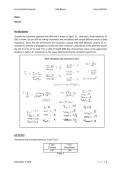
Consider the schematic captured from ADS that is shown in Figure 3.1. Note that a load impedance of
50Ω is shown, but you will be making calculations and simulations with several different values of load
impedance. Given that the transmission line comprises a coaxial cable with dielectric constant of 2.1,
calculate the velocity of propagation and the time that it takes for a disturbance at the generator end of
the line to arrive at the load T for a cable of length 1000 feet. Record these values in the appropriate
locations in Table 1 for comparison to the values obtained during the simulation experiment.
Show calculation steps and answers here.
Lab Section
Theoretical and Simulated Values of Travel Times:
𝑇 (𝜇𝑠) 𝑇 (𝜇𝑠)
(Theory) (Simulation)
1.47 1.44
Table 1
September 3, 2019 Page |1
, Arizona State University Lab2 Report iCourse EEE341
Theoretical and Simulated Values of Γ𝐿 :
𝑍𝐿 (Ω) Γ𝐿 Γ𝐿
(Theory) (Simulation)
infinity 1 0.998
100 0.333 0.332
50 0 0.0006
25 -0.333 -0.332
0 -1 -0.998
Table 2
Theoretical and Simulated Values of Pulse Amplitudes:
𝑍𝐿 (Ω) 𝑉𝑖𝑛𝑐 (𝑉) 𝑉𝑟𝑒𝑓 (𝑉) 𝑉𝑙𝑜𝑎𝑑 (𝑉) 𝑉𝑖𝑛𝑐 (𝑉) 𝑉𝑟𝑒𝑓 (𝑉) 𝑉𝑙𝑜𝑎𝑑 (𝑉)
(Theory) (Theory) (Theory) (Simulation) (Simulation) (Simulation)
infinity 0.5 0.5 1 0.500 0.499 0.999
100 0.5 0.1667 0.667 0.500 0.166 0.666
50 0.5 0 0.5 0.500 3.310*10-4 0.500
25 0.5 -0.1667 0.333 0.500 -0.166 0.333
0 0.5 -0.5 0 0.500 -0.499 0.00
Table 3
The graphs displaying the incident, reflected, and load pulses (10 total graphs)
𝑍𝐿 = ∞ (incident and reflected pulses):
Demonstrate the plot in this area.
September 3, 2019 Page |2
Name:
ASU ID:
Pre-lab Section
Consider the schematic captured from ADS that is shown in Figure 3.1. Note that a load impedance of
50Ω is shown, but you will be making calculations and simulations with several different values of load
impedance. Given that the transmission line comprises a coaxial cable with dielectric constant of 2.1,
calculate the velocity of propagation and the time that it takes for a disturbance at the generator end of
the line to arrive at the load T for a cable of length 1000 feet. Record these values in the appropriate
locations in Table 1 for comparison to the values obtained during the simulation experiment.
Show calculation steps and answers here.
Lab Section
Theoretical and Simulated Values of Travel Times:
𝑇 (𝜇𝑠) 𝑇 (𝜇𝑠)
(Theory) (Simulation)
1.47 1.44
Table 1
September 3, 2019 Page |1
, Arizona State University Lab2 Report iCourse EEE341
Theoretical and Simulated Values of Γ𝐿 :
𝑍𝐿 (Ω) Γ𝐿 Γ𝐿
(Theory) (Simulation)
infinity 1 0.998
100 0.333 0.332
50 0 0.0006
25 -0.333 -0.332
0 -1 -0.998
Table 2
Theoretical and Simulated Values of Pulse Amplitudes:
𝑍𝐿 (Ω) 𝑉𝑖𝑛𝑐 (𝑉) 𝑉𝑟𝑒𝑓 (𝑉) 𝑉𝑙𝑜𝑎𝑑 (𝑉) 𝑉𝑖𝑛𝑐 (𝑉) 𝑉𝑟𝑒𝑓 (𝑉) 𝑉𝑙𝑜𝑎𝑑 (𝑉)
(Theory) (Theory) (Theory) (Simulation) (Simulation) (Simulation)
infinity 0.5 0.5 1 0.500 0.499 0.999
100 0.5 0.1667 0.667 0.500 0.166 0.666
50 0.5 0 0.5 0.500 3.310*10-4 0.500
25 0.5 -0.1667 0.333 0.500 -0.166 0.333
0 0.5 -0.5 0 0.500 -0.499 0.00
Table 3
The graphs displaying the incident, reflected, and load pulses (10 total graphs)
𝑍𝐿 = ∞ (incident and reflected pulses):
Demonstrate the plot in this area.
September 3, 2019 Page |2

