
M&S 4
Introduction to Optimization Techniques
M&S 4 – Introduction to Optimization Techniques
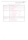
Subjects Subject Details
Linear Programming o Linear Programming (LP) Problem
o Graphical Method
Simplex Method - Simplex Tableau
- Simplex Method
- Big M Method
Network Problems Terminology of Network Problems
Transportation Problem (week 6)
o North-west Corner Method (week 6)
Shortest Path (week 6)
o Dijkstra’s Algorithm
o Hillier and Lieberman Method
Maximum Flow Problem (week 7)
Minimum Cost Problem (week 7)
Travelling Salesman Problem (week 8)
o Nearest Neighbor
Definitions - Terms with explanation (week 1 – week 8)
Templates (which can be 1. Simplex Tableau
used for the exam) 2. Dijkstra’s Algorithm
3. Hillier and Lieberman Method
4. Minimum Cost Flow Problem
5. Nearest Neighbor Algorithm
1
, M&S 4
Introduction to Optimization Techniques
Linear Programming
Linear Programming is maximizing or minimizing a linear goal
function subject to linear constraints.
The LP Problem is allocating limited resources among competing activities in a best possible
way.
For example. Hit the target by using maximum 3 arrows form minimal 5 meters distance.
Decision Variables
o Which units do you change in order to reach your objective?
o For example. x 1 , x 2
Objective Function
o Goal of the problem.
o Maximum or minimum.
o For example. Maximize profit or minimize costs.
Constraints
o Restrictions or limitations on the decision variables.
o For example. 5 x 1+ 9 x 2 ≤35 .
Steps in Linear Programming
1. Determine the variables.
2. Formulate the objective.
3. Write the constraints.
4. Solve the LP problem.
Linear Programming – Graphical Method
The graphical method is best explained using an example.
Acme Bicycle Company (ABC) produces two kinds of bicycles:
- Mountain bikes; profit €15 per bicycle. X1
- Street racers; profit €10 per bicycle. X2
Which amount of each type of bicycle should be produced to maximize profit?
Two teams of producers with maximum production rate: 2 mountain bikes per day and 3
street racers per day respectively.
Metal finishing machine requires the same amount of time for both type of bikes and can
produce in total 4 bikes per day, of either type.
1. Determine the variables.
x 1 = Amount of produced mountain bikes per day.
x 2 = Amount of produced street racers per day.
2. Give the objective function.
Maximum z=15 x 1+10 x 2.
3. Formulate the constraints.
x1 ≤ 2 Mountain bike production limit.
x2≤ 3 Street racers production limit.
x 1+ x2 ≤ 4 Metal finishing machine production limit.
x1, x2≥ 0 There can be no negative production.
2
, M&S 4
Introduction to Optimization Techniques
The limiting value of each constraint is shown as a line. Each constraint
eliminates part of the plan. See graph on the right.
Terminology solution space
Terminology for possible solutions:
o Feasible solution; all constraints are satisfied.
o Optimal solution; feasible solution with most favorable value
of the objective.
o Corner-point feasible (CPF) solution; solution at the corner of the feasible
region.
Find the optimum
The optimum is always a corner point. Two ways to find the optimum:
Option 1. Calculate the objective value for each CPF. The most favorable outcome of the
objective is the optimum.
a. Calculate the intersections of the constraints and their objective value.
Option 2. Use the objective line. The optimum is where the objective function
has only one point in the feasible region left when moving it from left to right.
1. Choose a random number. (Hint; choose an easy multiplier of both
coefficients.
For example. Objective z=15 x 1+10 x 2. Easy to multiplier is 30.
2. Draw the objective line for the chosen number.
For example. z (2,0 )=30∧z ( 0,3 )=3.
3. Shift the objective line such that the objective line touches only
one point of the feasible region, this will be the optimum.
For example. z (2,2 )=50.
Excel Solver - Brightspace
How to use the LP solver in Excel, see video on Brightspace.
3
, M&S 4
Introduction to Optimization Techniques
Special types of LP problems
1. Pure integer programming. All variables integer.
2. Mixed integer programming. Some but not all variables integer.
3. Binary integer programming. All variables are binary (0 or 1).
An integer solution can never be better than the LP solution and is usually a worse solution.
A rounded optimal solution of the non-integer problem is not necessary the optimal solution
of the integer problem. The graphical method does not always lead to the optimal integer
solution.
When integer programming in Excel, go to data tab Analyze group solver.
Example 1. Production parts
Step 1. Variables:
x 1 = Amount of produced parts A.
x 2 = Amount of produced parts B.
Step 2. Objective: Max. z=30 x 1+ 20 x 2
Step 3. Constraints:
2 x1 +1 x 2 ≤ 140 Max. available capacity for drilling.
1 x1 +2 x 2 ≤ 160 Max. available capacity for
1 x1 +1 x2 ≤ 900 Max. available capacity for
x1, x2≥ 0 There can be no negative production.
Example 2. Rolls Royce
Step 1. Variables:
x 1 = Number of aircraft engines.
x 2 = Number of train engines.
Step 2. Objective: Max. z=14 x 1 +12 x 2
Step 3. Constraints:
2 x1 +3 x 2 ≤ 12 Wiring hours production limit.
6 x 1+ 5 x 2 ≤30 Assembly hours production limit.
x1, x2≥ 0 There can be no negative production.
Example 3. Copier Machine
Step 1. Variables:
x 1 = Number of high-speed copiers.
x 2 = Number of low speed copiers.
Step 2. Objective: Min. z=6,000 x 1+ 4,000 x 2
Step 3. Constraints:
x 1+ x2 ≥6 At least six copiers.
x1≥ 1 At least one high speed copier.
20,000 x 1+10,000 x 2 ≥ 75,000 A and B need to handle at least 75,000 per day.
x1, x2≥ 0 There can be no negative production.
4
Introduction to Optimization Techniques
M&S 4 – Introduction to Optimization Techniques
Subjects Subject Details
Linear Programming o Linear Programming (LP) Problem
o Graphical Method
Simplex Method - Simplex Tableau
- Simplex Method
- Big M Method
Network Problems Terminology of Network Problems
Transportation Problem (week 6)
o North-west Corner Method (week 6)
Shortest Path (week 6)
o Dijkstra’s Algorithm
o Hillier and Lieberman Method
Maximum Flow Problem (week 7)
Minimum Cost Problem (week 7)
Travelling Salesman Problem (week 8)
o Nearest Neighbor
Definitions - Terms with explanation (week 1 – week 8)
Templates (which can be 1. Simplex Tableau
used for the exam) 2. Dijkstra’s Algorithm
3. Hillier and Lieberman Method
4. Minimum Cost Flow Problem
5. Nearest Neighbor Algorithm
1
, M&S 4
Introduction to Optimization Techniques
Linear Programming
Linear Programming is maximizing or minimizing a linear goal
function subject to linear constraints.
The LP Problem is allocating limited resources among competing activities in a best possible
way.
For example. Hit the target by using maximum 3 arrows form minimal 5 meters distance.
Decision Variables
o Which units do you change in order to reach your objective?
o For example. x 1 , x 2
Objective Function
o Goal of the problem.
o Maximum or minimum.
o For example. Maximize profit or minimize costs.
Constraints
o Restrictions or limitations on the decision variables.
o For example. 5 x 1+ 9 x 2 ≤35 .
Steps in Linear Programming
1. Determine the variables.
2. Formulate the objective.
3. Write the constraints.
4. Solve the LP problem.
Linear Programming – Graphical Method
The graphical method is best explained using an example.
Acme Bicycle Company (ABC) produces two kinds of bicycles:
- Mountain bikes; profit €15 per bicycle. X1
- Street racers; profit €10 per bicycle. X2
Which amount of each type of bicycle should be produced to maximize profit?
Two teams of producers with maximum production rate: 2 mountain bikes per day and 3
street racers per day respectively.
Metal finishing machine requires the same amount of time for both type of bikes and can
produce in total 4 bikes per day, of either type.
1. Determine the variables.
x 1 = Amount of produced mountain bikes per day.
x 2 = Amount of produced street racers per day.
2. Give the objective function.
Maximum z=15 x 1+10 x 2.
3. Formulate the constraints.
x1 ≤ 2 Mountain bike production limit.
x2≤ 3 Street racers production limit.
x 1+ x2 ≤ 4 Metal finishing machine production limit.
x1, x2≥ 0 There can be no negative production.
2
, M&S 4
Introduction to Optimization Techniques
The limiting value of each constraint is shown as a line. Each constraint
eliminates part of the plan. See graph on the right.
Terminology solution space
Terminology for possible solutions:
o Feasible solution; all constraints are satisfied.
o Optimal solution; feasible solution with most favorable value
of the objective.
o Corner-point feasible (CPF) solution; solution at the corner of the feasible
region.
Find the optimum
The optimum is always a corner point. Two ways to find the optimum:
Option 1. Calculate the objective value for each CPF. The most favorable outcome of the
objective is the optimum.
a. Calculate the intersections of the constraints and their objective value.
Option 2. Use the objective line. The optimum is where the objective function
has only one point in the feasible region left when moving it from left to right.
1. Choose a random number. (Hint; choose an easy multiplier of both
coefficients.
For example. Objective z=15 x 1+10 x 2. Easy to multiplier is 30.
2. Draw the objective line for the chosen number.
For example. z (2,0 )=30∧z ( 0,3 )=3.
3. Shift the objective line such that the objective line touches only
one point of the feasible region, this will be the optimum.
For example. z (2,2 )=50.
Excel Solver - Brightspace
How to use the LP solver in Excel, see video on Brightspace.
3
, M&S 4
Introduction to Optimization Techniques
Special types of LP problems
1. Pure integer programming. All variables integer.
2. Mixed integer programming. Some but not all variables integer.
3. Binary integer programming. All variables are binary (0 or 1).
An integer solution can never be better than the LP solution and is usually a worse solution.
A rounded optimal solution of the non-integer problem is not necessary the optimal solution
of the integer problem. The graphical method does not always lead to the optimal integer
solution.
When integer programming in Excel, go to data tab Analyze group solver.
Example 1. Production parts
Step 1. Variables:
x 1 = Amount of produced parts A.
x 2 = Amount of produced parts B.
Step 2. Objective: Max. z=30 x 1+ 20 x 2
Step 3. Constraints:
2 x1 +1 x 2 ≤ 140 Max. available capacity for drilling.
1 x1 +2 x 2 ≤ 160 Max. available capacity for
1 x1 +1 x2 ≤ 900 Max. available capacity for
x1, x2≥ 0 There can be no negative production.
Example 2. Rolls Royce
Step 1. Variables:
x 1 = Number of aircraft engines.
x 2 = Number of train engines.
Step 2. Objective: Max. z=14 x 1 +12 x 2
Step 3. Constraints:
2 x1 +3 x 2 ≤ 12 Wiring hours production limit.
6 x 1+ 5 x 2 ≤30 Assembly hours production limit.
x1, x2≥ 0 There can be no negative production.
Example 3. Copier Machine
Step 1. Variables:
x 1 = Number of high-speed copiers.
x 2 = Number of low speed copiers.
Step 2. Objective: Min. z=6,000 x 1+ 4,000 x 2
Step 3. Constraints:
x 1+ x2 ≥6 At least six copiers.
x1≥ 1 At least one high speed copier.
20,000 x 1+10,000 x 2 ≥ 75,000 A and B need to handle at least 75,000 per day.
x1, x2≥ 0 There can be no negative production.
4