EC2B5 notes
economic analysis to explore important questions in contemporary macroeconomic policy
Fiscal stimulus vs austerity
• How should governments deal with an unsustainable level of debt?
• Should debt reduction be front-loaded or phased in gradually?
• Did Greece make the right choice in their debt crisis?
Growth policy
• What drives convergence in income levels across countries?
• Why do some countries stay poor?
• What is the role of endogenous growth?
• What can governments do to promote growth?: The role of endogenous growth theory - maintains
that economic growth is primarily the result of internal forces, rather than external ones. It argues
that improvements in productivity can be tied directly to faster innovation and more investments in
human capital from governments and private sector institutions.
IS-LM model – assumptions: simplifies economy to good mkt and money mkt, prices are fixed
IS-LM (Investment saving-liquidity money supply) is a useful tool for:
understanding the effects of macroeconomic shocks (where the eqm moves to after a shock like covid)
• the role of policy in economic stabilisation
• it focusses on equilibrium behaviour of the economy in the short-run
• equilibrium is a state of rest, where there is no force in the economy acting for change.
Equilibrium in the economy requires both goods and money market are in equilibrium.
• IS curve represents goods market eqm:
determines equilibrium income/output (Y).
• LM curve represents money market eqm:
determines the equilibrium interest rate (r).
• Goods market equilibrium requires: aggregate supply (AS) = aggregate demand (AD)
• Aggregate demand consists of:
consumption (increasing in Y) increase consumer confidence
investment (decreasing in r)
government spending (fixed).
(exports-imports not included as ISLM closed economy – no trade)
• Graphical representation of IS curve:
represents all possible combinations of (Y,r) for which goods market is in
equilibrium
IS curve is downward-sloping as increase in interest, less investment,
less AD
Money market equilibrium
• Money market equilibrium requires: money supply = money demand
• Demand for money is derived from Keynes’ Liquidity Preference Theory:
Argues people hold money in order to undertake transactions (medium of exchange)
How much? increasing in Y: higher income means increased spending
decreasing in r: higher interest rate increases the opportunity cost of holding money.
• Money supply is fixed by the central bank: it is independent of the interest rate
• Money market equilibrium occurs at the intersection of the demand and supply
curves.
• Tip: if a variable is not represented on one of the axis eg income change in
variable=shift, if variable is represented on axis then change in variable =
movement on curve
• Suppose there is an increase in income MD to MD’:
money demand curve shifts outwards
inducing excess demand for money
hence r increases to restore equilibrium.
,LM curve
• Graphical representation of LM curve:
represents all possible combinations of (Y,r) for which
money market is in equilibrium
LM curve is upward-sloping – increase in income, increase
money demand, increase interest to restore eqm (+ve
relationship)
• Equilibrium in the economy requires both goods and money
markets are simultaneously in equilibrium.
Putting the two together
• This is known as general equilibrium.
• It is a unique equilibrium which occurs at the intersection of the IS and
LM curves.
• IS-LM is useful for understanding role of policy in stabilising economic
fluctuations:
fiscal policy: changes in government spending and taxes
monetary policy: changes in money supply.
• How does fiscal policy work?
• An increase in government spending (G) boosts aggregate
demand and income.
• The overall increase in income is larger than the initial
increase in G:
because the initial boost to income induces second
round effects on consumer spending, increase G,
more jobs, increase C (a to c)
this is called the Keynesian multiplier effect.
• Overall change in income is smaller than the full effect of the
Keynesian multiplier:
increase in income induces excess demand for money, hence interest rate increases
but this decreases investment spending which partially offsets the increase in aggregate
demand (a to b instead of c)
this is known as crowding out.
Crowding out reduces the effectiveness of fiscal policy as a tool of economic
stabilisation
Monetary policy: An expansion of the money supply - shifts LM curve to the
right, decreases interest rate & increases output
Induces excess supply of money which decreases interest rate, increases
investment spending, increases AD and income – known as interest rate channel
of monetary policy.
AD-AS model
AD-AS model also studies short run economic fluctuations and the role of policy.
Key shortcomings of IS-LM:
• prices are fixed
• the equilibrium level of output is determined purely by aggregate demand.
In AD-AS however:
• prices are flexible (therefore gives insights into inflation)
• aggregate supply also plays a role in determining the equilibrium level of output
– recessions caused for supply shocks too
AD-AS model focusses on the behaviour of two key variables: output/total GDP (Q), prices (P)
Consists of two key components:
AD curve: quantity of goods and services households want to buy at given prices
AS curve: quantity of goods and services firms want to produce at given prices.
,• Equilibrium in the economy occurs where: aggregate demand = aggregate supply
• Prices adjust in order to equate aggregate supply and demand:
so the economy converges back to equilibrium.
AD downward sloping – fall in price level causes expansion in AD
• The AS curve is upward-sloping in the SR – higher prices makes output more profitable and real
wages lower (profitable for firms)
• But in the long run:
AS curve becomes vertical.
AD, SRAS & LRAS all intersect.
Long run equilibrium
• In the LR, aggregate supply depends on the productive
potential of the economy: quantity/quality of factors of p
labour supply, capital stock and productivity.
• This fixed level of output in the long-run is known as the
natural rate of output.
• In the short-run, the economy might deviate from the natural
rate, e.g. recession:
but over time, wages and prices adjust
hence in the LR, the economy reverts back to the natural rate.
Contraction in money supply (attempts to
slow the economy by reducing the money
supply and fending off inflation by raising IRs):
AD curve shifts leftwards (firms see
unsold stock rise and cut their production)
prices and output fall
unemployment rises
hence the economy goes into recession
Fiscal expansion:
AD curve shifts right, prices and output increase, unemployment falls
Shifts in aggregate demand
Aggregate demand weak: prices falling (inflation low), output below natural rate (unemployment high)
Aggregate demand strong: prices rising (inflation high), output above natural rate (unemployment low)
• Hence, we observe an inverse relationship between inflation and
unemployment.
This inverse relationship is commonly known as the Phillips Curve.
• Government can boost aggregate demand in order to reduce
unemployment:
but this puts upward pressure on wages
hence firms increase prices and inflation increases.
• Thus, policymakers face an inevitable trade-off between inflation and
unemployment.
Hence, major importance for policymakers
have a choice between low inflation and low unemployment in the short
run.
• In the long run, there is no such trade-off between inflation and
unemployment.
• The LR Phillips Curve is vertical, where:
unemployment is fixed at the natural rate of
unemployment.
, The Case for Central Bank independence
-Up until 1997, the UK did not have an independent central bank
1979 Thatcher Government elected: key priority - low inflation
Monetarism - control of money supply growth:
“Inflation is always and everywhere a monetary phenomenon”
Policy successful in SR: Interest rates hit 17%, Inflation fell below 5% however u/e soared
1985 monetarism abandoned.
Late 1980s Lawson economic boom occurred.
1988 Thatcher re-elected.
However price to pay for this as 1990 inflation surged to 10%
-In LR no trade off between inflation and
unemployment (so govt cant reduce unemployment
below natural rate at this level)
So, what causes the SR Phillips curve to shift up?
-Workers need to form an expectation of future
inflation when negotiating wage increases.
An increase in inflation expectations leads to higher
inflation because:
-workers raise wage demands to maintain real wages
-firms’ labour costs increase, hence they push up prices and inflation
increases
-SR Phillips curve shifts upwards.
At the intersection of SRPC and LRPC, inflation expectations equal actual inflation where u/e is at natural
rate
Time inconsistency of monetary policy
Suppose the government controls monetary
policy and faces re-election in May 2024:
In the SR: Jan 2024: low inflation exp and
workers negotiate and fix wages (nominal
wage rigidity) at point A where SRPC=LRPC,
Feb 2024: govt. sets monetary policy and
against promise decides on expansionary
monetary policy to stimulate economy/AD by
reducing IRs to win election, ‘inflation surprise’ soares to point B, erosion of
real wages, firms real costs fall and take advantage by increasing production, hiring more and u/e falls
May 2024: u/e falls, inflation expectations remain low (due to adaptive expectations – exp only adjust
gradually) and govt win general election
In the LR: Jan 2025: workers renegotiate wages and now realise govt
caused inflation surprise, respond by increasing inflation
expectation, increase wage demands, inflation rises, SRPC shifts up
to point C (not pint D as only way to reduce u/e from natural rate is
through inflation surprise which erodes real wages)
-inflation has increased, but unemployment is unchanged.
Hence, there is no trade-off between inflation and
unemployment in the long run.
Overall, society is worse off from the pre-election boom: because
the economy is stuck in a high inflation equilibrium.
Policy credibility: Suppose the government again promises to stick to low inflation from now on: in order
to lower inflation expectations to move from point C to A
-Will the public believe them? No – the minute they lower inflation expectations, govt will take advantage
and take on another inflation surprise, eroding real wages leading to point B to win election again yet
public foresees this time and remain stuck with their inflation expecations remaining at point C.
economic analysis to explore important questions in contemporary macroeconomic policy
Fiscal stimulus vs austerity
• How should governments deal with an unsustainable level of debt?
• Should debt reduction be front-loaded or phased in gradually?
• Did Greece make the right choice in their debt crisis?
Growth policy
• What drives convergence in income levels across countries?
• Why do some countries stay poor?
• What is the role of endogenous growth?
• What can governments do to promote growth?: The role of endogenous growth theory - maintains
that economic growth is primarily the result of internal forces, rather than external ones. It argues
that improvements in productivity can be tied directly to faster innovation and more investments in
human capital from governments and private sector institutions.
IS-LM model – assumptions: simplifies economy to good mkt and money mkt, prices are fixed
IS-LM (Investment saving-liquidity money supply) is a useful tool for:
understanding the effects of macroeconomic shocks (where the eqm moves to after a shock like covid)
• the role of policy in economic stabilisation
• it focusses on equilibrium behaviour of the economy in the short-run
• equilibrium is a state of rest, where there is no force in the economy acting for change.
Equilibrium in the economy requires both goods and money market are in equilibrium.
• IS curve represents goods market eqm:
determines equilibrium income/output (Y).
• LM curve represents money market eqm:
determines the equilibrium interest rate (r).
• Goods market equilibrium requires: aggregate supply (AS) = aggregate demand (AD)
• Aggregate demand consists of:
consumption (increasing in Y) increase consumer confidence
investment (decreasing in r)
government spending (fixed).
(exports-imports not included as ISLM closed economy – no trade)
• Graphical representation of IS curve:
represents all possible combinations of (Y,r) for which goods market is in
equilibrium
IS curve is downward-sloping as increase in interest, less investment,
less AD
Money market equilibrium
• Money market equilibrium requires: money supply = money demand
• Demand for money is derived from Keynes’ Liquidity Preference Theory:
Argues people hold money in order to undertake transactions (medium of exchange)
How much? increasing in Y: higher income means increased spending
decreasing in r: higher interest rate increases the opportunity cost of holding money.
• Money supply is fixed by the central bank: it is independent of the interest rate
• Money market equilibrium occurs at the intersection of the demand and supply
curves.
• Tip: if a variable is not represented on one of the axis eg income change in
variable=shift, if variable is represented on axis then change in variable =
movement on curve
• Suppose there is an increase in income MD to MD’:
money demand curve shifts outwards
inducing excess demand for money
hence r increases to restore equilibrium.
,LM curve
• Graphical representation of LM curve:
represents all possible combinations of (Y,r) for which
money market is in equilibrium
LM curve is upward-sloping – increase in income, increase
money demand, increase interest to restore eqm (+ve
relationship)
• Equilibrium in the economy requires both goods and money
markets are simultaneously in equilibrium.
Putting the two together
• This is known as general equilibrium.
• It is a unique equilibrium which occurs at the intersection of the IS and
LM curves.
• IS-LM is useful for understanding role of policy in stabilising economic
fluctuations:
fiscal policy: changes in government spending and taxes
monetary policy: changes in money supply.
• How does fiscal policy work?
• An increase in government spending (G) boosts aggregate
demand and income.
• The overall increase in income is larger than the initial
increase in G:
because the initial boost to income induces second
round effects on consumer spending, increase G,
more jobs, increase C (a to c)
this is called the Keynesian multiplier effect.
• Overall change in income is smaller than the full effect of the
Keynesian multiplier:
increase in income induces excess demand for money, hence interest rate increases
but this decreases investment spending which partially offsets the increase in aggregate
demand (a to b instead of c)
this is known as crowding out.
Crowding out reduces the effectiveness of fiscal policy as a tool of economic
stabilisation
Monetary policy: An expansion of the money supply - shifts LM curve to the
right, decreases interest rate & increases output
Induces excess supply of money which decreases interest rate, increases
investment spending, increases AD and income – known as interest rate channel
of monetary policy.
AD-AS model
AD-AS model also studies short run economic fluctuations and the role of policy.
Key shortcomings of IS-LM:
• prices are fixed
• the equilibrium level of output is determined purely by aggregate demand.
In AD-AS however:
• prices are flexible (therefore gives insights into inflation)
• aggregate supply also plays a role in determining the equilibrium level of output
– recessions caused for supply shocks too
AD-AS model focusses on the behaviour of two key variables: output/total GDP (Q), prices (P)
Consists of two key components:
AD curve: quantity of goods and services households want to buy at given prices
AS curve: quantity of goods and services firms want to produce at given prices.
,• Equilibrium in the economy occurs where: aggregate demand = aggregate supply
• Prices adjust in order to equate aggregate supply and demand:
so the economy converges back to equilibrium.
AD downward sloping – fall in price level causes expansion in AD
• The AS curve is upward-sloping in the SR – higher prices makes output more profitable and real
wages lower (profitable for firms)
• But in the long run:
AS curve becomes vertical.
AD, SRAS & LRAS all intersect.
Long run equilibrium
• In the LR, aggregate supply depends on the productive
potential of the economy: quantity/quality of factors of p
labour supply, capital stock and productivity.
• This fixed level of output in the long-run is known as the
natural rate of output.
• In the short-run, the economy might deviate from the natural
rate, e.g. recession:
but over time, wages and prices adjust
hence in the LR, the economy reverts back to the natural rate.
Contraction in money supply (attempts to
slow the economy by reducing the money
supply and fending off inflation by raising IRs):
AD curve shifts leftwards (firms see
unsold stock rise and cut their production)
prices and output fall
unemployment rises
hence the economy goes into recession
Fiscal expansion:
AD curve shifts right, prices and output increase, unemployment falls
Shifts in aggregate demand
Aggregate demand weak: prices falling (inflation low), output below natural rate (unemployment high)
Aggregate demand strong: prices rising (inflation high), output above natural rate (unemployment low)
• Hence, we observe an inverse relationship between inflation and
unemployment.
This inverse relationship is commonly known as the Phillips Curve.
• Government can boost aggregate demand in order to reduce
unemployment:
but this puts upward pressure on wages
hence firms increase prices and inflation increases.
• Thus, policymakers face an inevitable trade-off between inflation and
unemployment.
Hence, major importance for policymakers
have a choice between low inflation and low unemployment in the short
run.
• In the long run, there is no such trade-off between inflation and
unemployment.
• The LR Phillips Curve is vertical, where:
unemployment is fixed at the natural rate of
unemployment.
, The Case for Central Bank independence
-Up until 1997, the UK did not have an independent central bank
1979 Thatcher Government elected: key priority - low inflation
Monetarism - control of money supply growth:
“Inflation is always and everywhere a monetary phenomenon”
Policy successful in SR: Interest rates hit 17%, Inflation fell below 5% however u/e soared
1985 monetarism abandoned.
Late 1980s Lawson economic boom occurred.
1988 Thatcher re-elected.
However price to pay for this as 1990 inflation surged to 10%
-In LR no trade off between inflation and
unemployment (so govt cant reduce unemployment
below natural rate at this level)
So, what causes the SR Phillips curve to shift up?
-Workers need to form an expectation of future
inflation when negotiating wage increases.
An increase in inflation expectations leads to higher
inflation because:
-workers raise wage demands to maintain real wages
-firms’ labour costs increase, hence they push up prices and inflation
increases
-SR Phillips curve shifts upwards.
At the intersection of SRPC and LRPC, inflation expectations equal actual inflation where u/e is at natural
rate
Time inconsistency of monetary policy
Suppose the government controls monetary
policy and faces re-election in May 2024:
In the SR: Jan 2024: low inflation exp and
workers negotiate and fix wages (nominal
wage rigidity) at point A where SRPC=LRPC,
Feb 2024: govt. sets monetary policy and
against promise decides on expansionary
monetary policy to stimulate economy/AD by
reducing IRs to win election, ‘inflation surprise’ soares to point B, erosion of
real wages, firms real costs fall and take advantage by increasing production, hiring more and u/e falls
May 2024: u/e falls, inflation expectations remain low (due to adaptive expectations – exp only adjust
gradually) and govt win general election
In the LR: Jan 2025: workers renegotiate wages and now realise govt
caused inflation surprise, respond by increasing inflation
expectation, increase wage demands, inflation rises, SRPC shifts up
to point C (not pint D as only way to reduce u/e from natural rate is
through inflation surprise which erodes real wages)
-inflation has increased, but unemployment is unchanged.
Hence, there is no trade-off between inflation and
unemployment in the long run.
Overall, society is worse off from the pre-election boom: because
the economy is stuck in a high inflation equilibrium.
Policy credibility: Suppose the government again promises to stick to low inflation from now on: in order
to lower inflation expectations to move from point C to A
-Will the public believe them? No – the minute they lower inflation expectations, govt will take advantage
and take on another inflation surprise, eroding real wages leading to point B to win election again yet
public foresees this time and remain stuck with their inflation expecations remaining at point C.