Week 1 -- Preparation
Field p.419-426
7.4 Bivariate correlation
7.4.4. Kendall's tau (non-parametric)
Kendall’s tau, T, is a non-parametric correlation and it should be used rather than Spearman’s
coefficient when you have a small data set with a large number of tied ranks (= if you rank all the
scores and many scores have the same rank).
To carry this out, follow the same steps as for Pearson and Spearman correlations but select
[Kendall’s tau-b].
Kendall’s value is a more accurate gauge of what the correlation in the population would be
(compared to Spearman).
7.4.5 Biserial and point-biserial correlations
These correlation coefficients are used when one of the two variables is dichotomous (i.e., it is
categorical with only two categories. E.g. being pregnant). The difference between the use of biserial
and point-biserial correlations depends on whether the dichotomous variable is discrete or continuous.
A discrete, or true, dichotomy is one for which there is no underlying continuum between the
categories (example = being dead).
It is possible to have a dichotomy for which a continuum does exist. An example is passing or failing
a test: some people will only just fail, while others will fail by a large margin. So although
participants fall into only two categories, there is an underlying continuum along which they lie.
The point-biserial correlation coefficient (rpb) is used when one variable is a discrete dichotomy,
whereas the biserial correlation coefficient (rb) is used when one variable is a continuous
dichotomy. The biserial coefficient cannot be calculated directly in SPSS; first you must calculate the
point-biserial correlation coefficient and then use an equation to adjust it.
A point-biserial correlation coefficient is simply a Pearson correlation when the dichotomous variable
is coded with 0 for one category and 1 for the other. The significance test for this correlation is
actually the same as performing an independent-samples t-test on the data. The sign of the coefficient
is completely dependent on which category you assign to which code and so we must ignore all
information about the direction of the relationship.
We can still interpret R^2. If R^2 = .378 = .143, we can conclude that gender accounts for 14.3% of
the variability in time spent away from home.
SUMMARY on correlations
● We can measure the relationship between two variables using correlation coefficients.
● These coefficients lie between -1 and +1.
● Pearson’s correlation coefficient, r, is a parametric statistic and requires interval data for both
variables. To test its significance we assume normality too.
● Spearman’s correlation coefficient, rs, is a non-parametric statistic and requires only ordinal
data for both variables.
● Kendall’s correlation coefficient, T, is like Spearman’s rs, but probably better for small
samples.
● The point-biserial correlation coefficient, rpb, quantifies the relationship between a continuous
variable and a variable that is a discrete dichotomy (e.g., there is no continuum underlying the
two categories).
, ● The biserial correlation coefficient, rb, quantifies the relationship between a continuous
variable and a variable that is a continuous dichotomy (e.g., there is a continuum underlying
the two categories, such as passing or failing an exam).
7.5 The partial correlation
7.5.1 The theory behind part and partial correlation
A correlation between two variables in which the effects of other variables are held constant is known
as a partial correlation.
We use partial correlations to find out the size of the unique portion of variance. Therefore, we could
conduct a partial correlation between exam anxiety and exam performance while ‘controlling’ for the
effect of revision time. Likewise, we could carry out a partial correlation between revision time and
exam performance while ‘controlling’ for the effects of exam anxiety.
Video lectures
Week 1.1 Introduction to the course
This video:
I. Introduction of the course.
II. Course outline.
A. Week 1 → Revision and categorical predictors.
B. Week 2 → Moderation.
C. Week 3 → Mediation.
D. Week 4 → ANOVA part 1: One-way ANOVA, ANCOVA, Fact, ANOVA.
, E. Week 5 → ANOVA part 2: RM ANOVA, MD ANOVA.
F. Week 6 → Logistic regression.
Week 1.2 Revision: linear regression
This video
● Intuition simple and multiple regression.
● Calculate test statistics regression.
● Interpret regression output.
Linear regression
= We are trying to model the relationship between a dependent variable (y) and multiple independent
variable(s) (x). Predicting y using x. How much y increases/decreases as a function of x.
General linear regression model =
Some part we can never predict is the random error.
b’s
We can calculate b0 and b1 for simple linear regression
- But often we let SPSS do the work for us, especially with multiple regression.
SPSS: Analyze → Regression → Linear. Pick dependent (exam score) and independent variables
(fear of stats). Click Go.
Constant B = b0.
Fear of stats B = b1.
Model fit
Suppose we have the coefficients:
→ How do we assess model fit? Are we making a poor or a good prediction?
Estimate ε
- If we estimate ε, we get a sense of how well our model can predict the DV from the IV.
- We can compare the amount of error of our model (SSR) to the error of a model with no
relationship between x and y (SST).
- We look at the differences between the regression line and the actual observations and add
these up.
- Low error ⇒ the model is good.
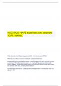
SST visualized (sum of squared total)
, Doesn’t take any information into account that you have on predicting exam scores.
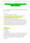
SSR visualized (sum of squared residual)
Where Yhead is the predicted value we got from our regression model.
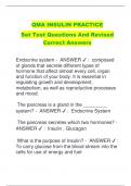
SSM visualized (sum of squared model)
In other words
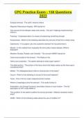
Formulas
Field p.419-426
7.4 Bivariate correlation
7.4.4. Kendall's tau (non-parametric)
Kendall’s tau, T, is a non-parametric correlation and it should be used rather than Spearman’s
coefficient when you have a small data set with a large number of tied ranks (= if you rank all the
scores and many scores have the same rank).
To carry this out, follow the same steps as for Pearson and Spearman correlations but select
[Kendall’s tau-b].
Kendall’s value is a more accurate gauge of what the correlation in the population would be
(compared to Spearman).
7.4.5 Biserial and point-biserial correlations
These correlation coefficients are used when one of the two variables is dichotomous (i.e., it is
categorical with only two categories. E.g. being pregnant). The difference between the use of biserial
and point-biserial correlations depends on whether the dichotomous variable is discrete or continuous.
A discrete, or true, dichotomy is one for which there is no underlying continuum between the
categories (example = being dead).
It is possible to have a dichotomy for which a continuum does exist. An example is passing or failing
a test: some people will only just fail, while others will fail by a large margin. So although
participants fall into only two categories, there is an underlying continuum along which they lie.
The point-biserial correlation coefficient (rpb) is used when one variable is a discrete dichotomy,
whereas the biserial correlation coefficient (rb) is used when one variable is a continuous
dichotomy. The biserial coefficient cannot be calculated directly in SPSS; first you must calculate the
point-biserial correlation coefficient and then use an equation to adjust it.
A point-biserial correlation coefficient is simply a Pearson correlation when the dichotomous variable
is coded with 0 for one category and 1 for the other. The significance test for this correlation is
actually the same as performing an independent-samples t-test on the data. The sign of the coefficient
is completely dependent on which category you assign to which code and so we must ignore all
information about the direction of the relationship.
We can still interpret R^2. If R^2 = .378 = .143, we can conclude that gender accounts for 14.3% of
the variability in time spent away from home.
SUMMARY on correlations
● We can measure the relationship between two variables using correlation coefficients.
● These coefficients lie between -1 and +1.
● Pearson’s correlation coefficient, r, is a parametric statistic and requires interval data for both
variables. To test its significance we assume normality too.
● Spearman’s correlation coefficient, rs, is a non-parametric statistic and requires only ordinal
data for both variables.
● Kendall’s correlation coefficient, T, is like Spearman’s rs, but probably better for small
samples.
● The point-biserial correlation coefficient, rpb, quantifies the relationship between a continuous
variable and a variable that is a discrete dichotomy (e.g., there is no continuum underlying the
two categories).
, ● The biserial correlation coefficient, rb, quantifies the relationship between a continuous
variable and a variable that is a continuous dichotomy (e.g., there is a continuum underlying
the two categories, such as passing or failing an exam).
7.5 The partial correlation
7.5.1 The theory behind part and partial correlation
A correlation between two variables in which the effects of other variables are held constant is known
as a partial correlation.
We use partial correlations to find out the size of the unique portion of variance. Therefore, we could
conduct a partial correlation between exam anxiety and exam performance while ‘controlling’ for the
effect of revision time. Likewise, we could carry out a partial correlation between revision time and
exam performance while ‘controlling’ for the effects of exam anxiety.
Video lectures
Week 1.1 Introduction to the course
This video:
I. Introduction of the course.
II. Course outline.
A. Week 1 → Revision and categorical predictors.
B. Week 2 → Moderation.
C. Week 3 → Mediation.
D. Week 4 → ANOVA part 1: One-way ANOVA, ANCOVA, Fact, ANOVA.
, E. Week 5 → ANOVA part 2: RM ANOVA, MD ANOVA.
F. Week 6 → Logistic regression.
Week 1.2 Revision: linear regression
This video
● Intuition simple and multiple regression.
● Calculate test statistics regression.
● Interpret regression output.
Linear regression
= We are trying to model the relationship between a dependent variable (y) and multiple independent
variable(s) (x). Predicting y using x. How much y increases/decreases as a function of x.
General linear regression model =
Some part we can never predict is the random error.
b’s
We can calculate b0 and b1 for simple linear regression
- But often we let SPSS do the work for us, especially with multiple regression.
SPSS: Analyze → Regression → Linear. Pick dependent (exam score) and independent variables
(fear of stats). Click Go.
Constant B = b0.
Fear of stats B = b1.
Model fit
Suppose we have the coefficients:
→ How do we assess model fit? Are we making a poor or a good prediction?
Estimate ε
- If we estimate ε, we get a sense of how well our model can predict the DV from the IV.
- We can compare the amount of error of our model (SSR) to the error of a model with no
relationship between x and y (SST).
- We look at the differences between the regression line and the actual observations and add
these up.
- Low error ⇒ the model is good.
SST visualized (sum of squared total)
, Doesn’t take any information into account that you have on predicting exam scores.
SSR visualized (sum of squared residual)
Where Yhead is the predicted value we got from our regression model.
SSM visualized (sum of squared model)
In other words
Formulas