1
Applications of Multiple Integrals
Recall from first year calculus that the average value of a real-valued
function, 𝑓(𝑥), on an interval [𝑎, 𝑏] is defined to be:
𝑏
1
𝑓𝐴𝑉𝐸 = ∫ 𝑓 (𝑥 )𝑑𝑥
𝑏−𝑎 𝑎
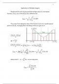
This comes from taking the value of the function 𝑓(𝑥) at 𝑛 equally spaced
points on [𝑎, 𝑏], averaging them and taking a limit as 𝑛 goes to ∞.
𝑦 = 𝑓(𝑥)
𝑓𝐴𝑉𝐸
𝑓(𝑥1 )+⋯+𝑓(𝑥𝑛 )
𝑛
𝑏−𝑎
∆𝑥 = 𝑎 = 𝑥0 𝑏 = 𝑥𝑛
𝑛
𝑓(𝑥1 )+⋯+𝑓(𝑥𝑛 ) ∆𝑥
= (𝑓 (𝑥1 ) + ⋯ + 𝑓(𝑥𝑛 )) 𝑏−𝑎
𝑛
𝑛
𝑏
1 1
𝑓𝐴𝑉𝐸 = lim ( ) ∑ 𝑓(𝑥𝑖 ) ∆𝑥 = ∫ 𝑓(𝑥) 𝑑𝑥
𝑛→∞ 𝑏 − 𝑎 𝑏−𝑎 𝑎
𝑖=1
𝑏
Notice that 𝑏 − 𝑎 = ∫𝑎 𝑑𝑥 , so we could write:
𝑏
∫𝑎 𝑓(𝑥 ) 𝑑𝑥
𝑓𝐴𝑉𝐸 = 𝑏 .
∫𝑎 𝑑𝑥
, 2
Similarly, we define the average of a real-valued function over a region 𝐷 ⊆ ℝ2
or a region 𝑊 ⊆ ℝ3 by:
∬𝐷 𝑓 (𝑥, 𝑦)𝑑𝑥 𝑑𝑦
𝑓𝐴𝑉𝐸 =
∬𝐷 𝑑𝑥 𝑑𝑦
∭𝑊 𝑓 (𝑥, 𝑦, 𝑧)𝑑𝑥 𝑑𝑦 𝑑𝑧
𝑓𝐴𝑉𝐸 =
∭𝑊 𝑑𝑥 𝑑𝑦 𝑑𝑧
Notice that the denominators are the area of 𝐷 and the volume of 𝑊,
respectively.
Ex. Find the average value of 𝑓 (𝑥, 𝑦) = 𝑥 sin(𝑥𝑦) on the region,
𝜋
𝐷 = [0, ] × [0, 𝜋].
2
𝜋
𝑦=𝜋 𝑥=
2
∬ 𝑓(𝑥, 𝑦)𝑑𝑥 𝑑𝑦 = ∫ ∫ (𝑥 sin(𝑥𝑦)) 𝑑𝑥 𝑑𝑦
𝐷 𝑦=0 𝑥=0
This is much easier to calculate if we reverse the order of integration:
𝜋 𝜋 𝑦=𝜋
𝑥= 2 𝑦=𝜋 𝑥= 2
=∫ ∫ (𝑥 sin(𝑥𝑦)) 𝑑𝑦 𝑑𝑥 = ∫ − cos(𝑥𝑦)| 𝑑𝑥
𝑥=0 𝑦=0 𝑥=0
𝑦=0
𝜋 𝜋
𝑥= 2 𝑥= 2
− sin(𝜋𝑥 )
=∫ (− cos(𝜋𝑥 ) + 1) 𝑑𝑥 = + 𝑥|
𝑥=0 𝜋 𝑥=0
𝜋2
− sin( ) 𝜋
2
= +2
𝜋
Applications of Multiple Integrals
Recall from first year calculus that the average value of a real-valued
function, 𝑓(𝑥), on an interval [𝑎, 𝑏] is defined to be:
𝑏
1
𝑓𝐴𝑉𝐸 = ∫ 𝑓 (𝑥 )𝑑𝑥
𝑏−𝑎 𝑎
This comes from taking the value of the function 𝑓(𝑥) at 𝑛 equally spaced
points on [𝑎, 𝑏], averaging them and taking a limit as 𝑛 goes to ∞.
𝑦 = 𝑓(𝑥)
𝑓𝐴𝑉𝐸
𝑓(𝑥1 )+⋯+𝑓(𝑥𝑛 )
𝑛
𝑏−𝑎
∆𝑥 = 𝑎 = 𝑥0 𝑏 = 𝑥𝑛
𝑛
𝑓(𝑥1 )+⋯+𝑓(𝑥𝑛 ) ∆𝑥
= (𝑓 (𝑥1 ) + ⋯ + 𝑓(𝑥𝑛 )) 𝑏−𝑎
𝑛
𝑛
𝑏
1 1
𝑓𝐴𝑉𝐸 = lim ( ) ∑ 𝑓(𝑥𝑖 ) ∆𝑥 = ∫ 𝑓(𝑥) 𝑑𝑥
𝑛→∞ 𝑏 − 𝑎 𝑏−𝑎 𝑎
𝑖=1
𝑏
Notice that 𝑏 − 𝑎 = ∫𝑎 𝑑𝑥 , so we could write:
𝑏
∫𝑎 𝑓(𝑥 ) 𝑑𝑥
𝑓𝐴𝑉𝐸 = 𝑏 .
∫𝑎 𝑑𝑥
, 2
Similarly, we define the average of a real-valued function over a region 𝐷 ⊆ ℝ2
or a region 𝑊 ⊆ ℝ3 by:
∬𝐷 𝑓 (𝑥, 𝑦)𝑑𝑥 𝑑𝑦
𝑓𝐴𝑉𝐸 =
∬𝐷 𝑑𝑥 𝑑𝑦
∭𝑊 𝑓 (𝑥, 𝑦, 𝑧)𝑑𝑥 𝑑𝑦 𝑑𝑧
𝑓𝐴𝑉𝐸 =
∭𝑊 𝑑𝑥 𝑑𝑦 𝑑𝑧
Notice that the denominators are the area of 𝐷 and the volume of 𝑊,
respectively.
Ex. Find the average value of 𝑓 (𝑥, 𝑦) = 𝑥 sin(𝑥𝑦) on the region,
𝜋
𝐷 = [0, ] × [0, 𝜋].
2
𝜋
𝑦=𝜋 𝑥=
2
∬ 𝑓(𝑥, 𝑦)𝑑𝑥 𝑑𝑦 = ∫ ∫ (𝑥 sin(𝑥𝑦)) 𝑑𝑥 𝑑𝑦
𝐷 𝑦=0 𝑥=0
This is much easier to calculate if we reverse the order of integration:
𝜋 𝜋 𝑦=𝜋
𝑥= 2 𝑦=𝜋 𝑥= 2
=∫ ∫ (𝑥 sin(𝑥𝑦)) 𝑑𝑦 𝑑𝑥 = ∫ − cos(𝑥𝑦)| 𝑑𝑥
𝑥=0 𝑦=0 𝑥=0
𝑦=0
𝜋 𝜋
𝑥= 2 𝑥= 2
− sin(𝜋𝑥 )
=∫ (− cos(𝜋𝑥 ) + 1) 𝑑𝑥 = + 𝑥|
𝑥=0 𝜋 𝑥=0
𝜋2
− sin( ) 𝜋
2
= +2
𝜋