my third stat assignment
oyakhire osose
2023-03-15
Exercise 10.12
The graph doesnt show a good comparison.Bar graph would have been preffered, even thought the height of each cone
represent the interest rate , each cone has differing width as well as the graph lacks the presence of an explanatory variable.
Exercise 10.14
we dont need other catgories as werent provided the data and should avoid making generalizations of the data
rates of students in the US from other countries
countries Rates
China 33.2%
India 17.9%
south Korea 5.0%
Saudi Arabia 4.1%
Canada 2.4%
rates <- c(33.2, 17.9,5.0,4.1,2.4,1.4)
> countries <-c ("china", "india", "southkorea", "SA", "canada","mexico")
> barplot(rates,names.arg = countries,main = "rates of students in the US from other countries")
exercise 10.28
, b. the overall pattern of the graph or trend is a longterm downward movement overtime
c. seasonal variations that were noted between 2008and 2014
years <-c(2000:2017)
count <-c(32562,28202,27229,25989,24373,24722,23739,21809,22401,18601,19486,19717,20144,19128,16539,16931,
15500,13956)
plot(data.frame(years, count), type = "l", main="line graph showing changes in time") # Equivalent
oyakhire osose
2023-03-15
Exercise 10.12
The graph doesnt show a good comparison.Bar graph would have been preffered, even thought the height of each cone
represent the interest rate , each cone has differing width as well as the graph lacks the presence of an explanatory variable.
Exercise 10.14
we dont need other catgories as werent provided the data and should avoid making generalizations of the data
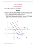
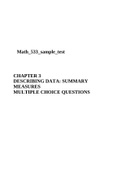
rates of students in the US from other countries
countries Rates
China 33.2%
India 17.9%
south Korea 5.0%
Saudi Arabia 4.1%
Canada 2.4%
rates <- c(33.2, 17.9,5.0,4.1,2.4,1.4)
> countries <-c ("china", "india", "southkorea", "SA", "canada","mexico")
> barplot(rates,names.arg = countries,main = "rates of students in the US from other countries")
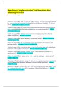
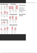
exercise 10.28
, b. the overall pattern of the graph or trend is a longterm downward movement overtime
c. seasonal variations that were noted between 2008and 2014
years <-c(2000:2017)
count <-c(32562,28202,27229,25989,24373,24722,23739,21809,22401,18601,19486,19717,20144,19128,16539,16931,
15500,13956)
plot(data.frame(years, count), type = "l", main="line graph showing changes in time") # Equivalent